Parameter Search

Solving problems with constraint conditions by Ising solvers (SA, SQA, etc,.) needs some techniques in the treatment of the constraint conditions. In this chapter, we explain the way to obtain feasible solutions, which satisfy all the constraint conditions, for these types of problems. This method is generally called the "parameter search".

Overview with Simple Example

In this section, we explain the parameter search with the simple example of the following problem.

$${\rm min} -x_0 - 2x_1 - 3x_2\\ {\rm subject\;to\;}x_0+x_1+x_2 = 1,\\ x_0,x_1,x_2\in\{0,1\} \tag{1}$$

One way to solve this problem by the Ising solvers is to convert the constraint condition to a penalty term like,

$${\rm min} f(x_0,x_1,x_2)\\ f(x_0,x_1,x_2)=-x_0 - 2x_1 - 3x_2 + \lambda\left(x_0+x_1+x_2 - 1\right)^2,\;\;\;0\leq\lambda \tag{2}$$

We here introduce the undetermined multiplier $\lambda\geq 0$, what we call the "parameter", to obtain feasible solutions. Let us now consider the effects of the penalty term $\lambda\left(x_0+x_1+x_2 - 1\right)^2$. When $\lambda=0$, the objective function is $-x_0 - 2x_1 - 3x_2$ and the optimal solution is obviously $(x_0,x_1,x_2)=(1,1,1)$, which dose not satisfy the constraint condition $x_0+x_1+x_2 = 1$. In contrast, sufficiently large $\lambda$ causes to change the optimal solution from $(x_0,x_1,x_2)=(1,1,1)$ to $(x_0,x_1,x_2)=(0,0,1)$. We can check this by write down all the possible solutions.

Table 1: All the possible solutions for the optimization problem [Eq. (2)].

State Number	$\boldsymbol{(x_0,x_1,x_2)}$	$\boldsymbol{f(x_0,x_1,x_2)}$	-
0	$(0,0,0)$	$\lambda$	infeasible
1	$(0,0,1)$	$-3$	feasible
2	$(0,1,0)$	$-2$	feasible
3	$(0,1,1)$	$\lambda-5$	infeasible
4	$(1,0,0)$	$-1$	feasible
5	$(1,0,1)$	$\lambda-4$	infeasible
6	$(1,1,0)$	$\lambda-3$	infeasible
7	$(1,1,1)$	$4\lambda-6$	infeasible

From this table, one can understand that the optimal solution for $\lambda=0$ is $(1,1,1)$. Comparing the two states $(0,1,1)$ and $(0,0,1)$, we can see that the optimal solution for $\lambda>2$ is $(0,0,1)$. The figures below show this situation by plotting the objective values for each state, what is called energy landscape.

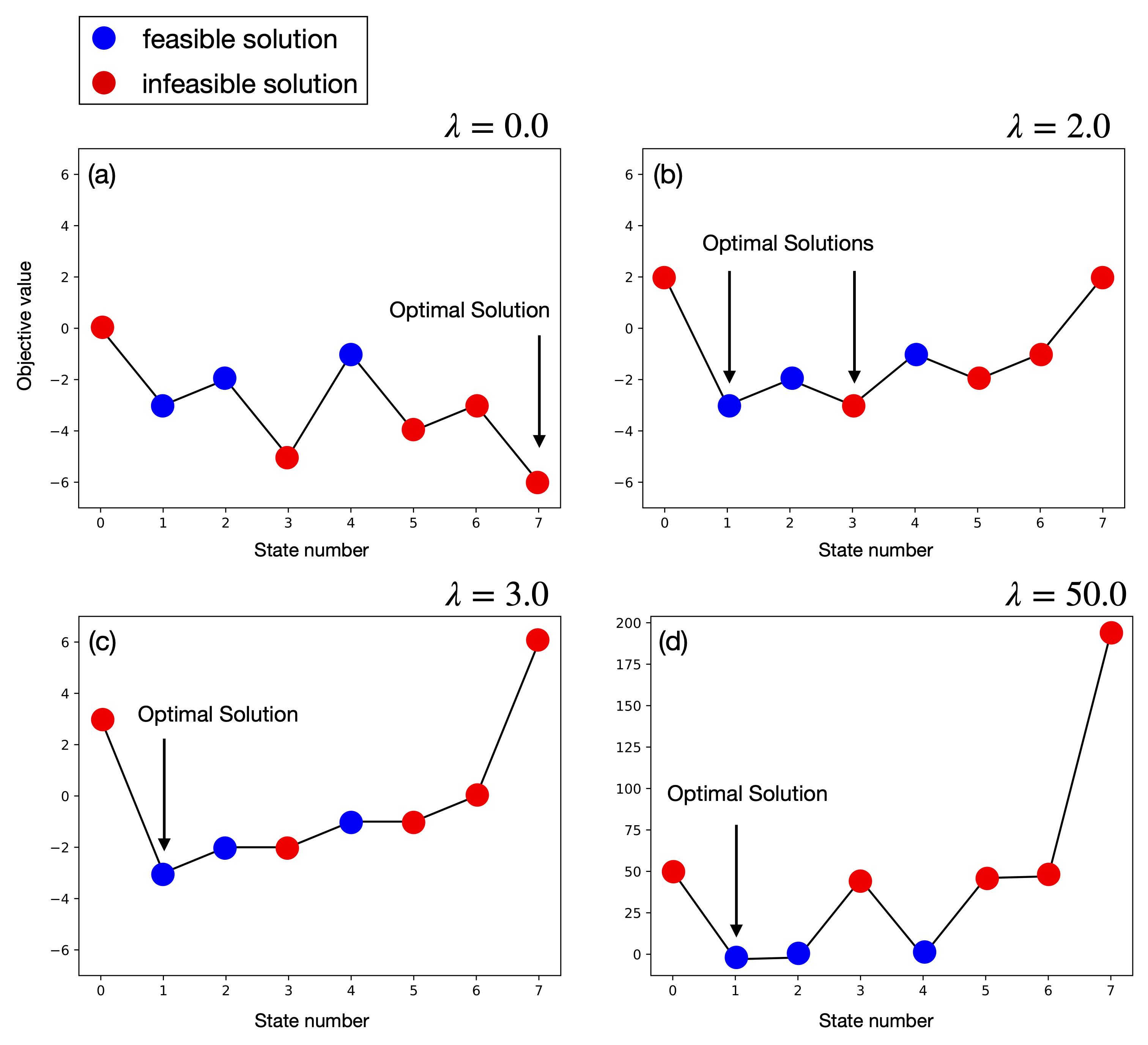Figure 1: Energy landscape for the objective function in Eq. (2) for (a) $\lambda=0.0$, (b) $\lambda=2.0$, (c) $\lambda=3.0$, and (d) $\lambda=50.0$.

The blue and red circles represent the feasible and infeasible solution respectively. The range of y-axis is the same for Fig. 1(a)-(c), and one can see that the objective values for infeasible solutions increase as $\lambda$ does. Figure 1(a) corresponds the $\lambda=0$ and the optimal solution is the state number 7 $(x_0,x_1,x_2)=(1,1,1)$, which is infeasible solution. When $\lambda=2$, the objective values of the feasible solution $(0,0,1)$ and the infeasible solution $(0,1,1)$ have the same value [Fig. 1(b)], and both two states are optimal. Thus, we can conclude that $\lambda$ must be larger than $2$ to obtain the feasible solution. Figure 1(c) corresponds to $\lambda=3$ and the optimal solution is only $(0,0,1)$. We note that too large $\lambda$ may lead to bad feasible solutions, since only the penalty term is dominant in Eq. (2). For example, in the case of $\lambda=50$ [Fig. 1(d)], Ising solvers may not distinguish all the feasible solutions, leading to obtain feasible but not optimal solutions.

Solve with JijZept

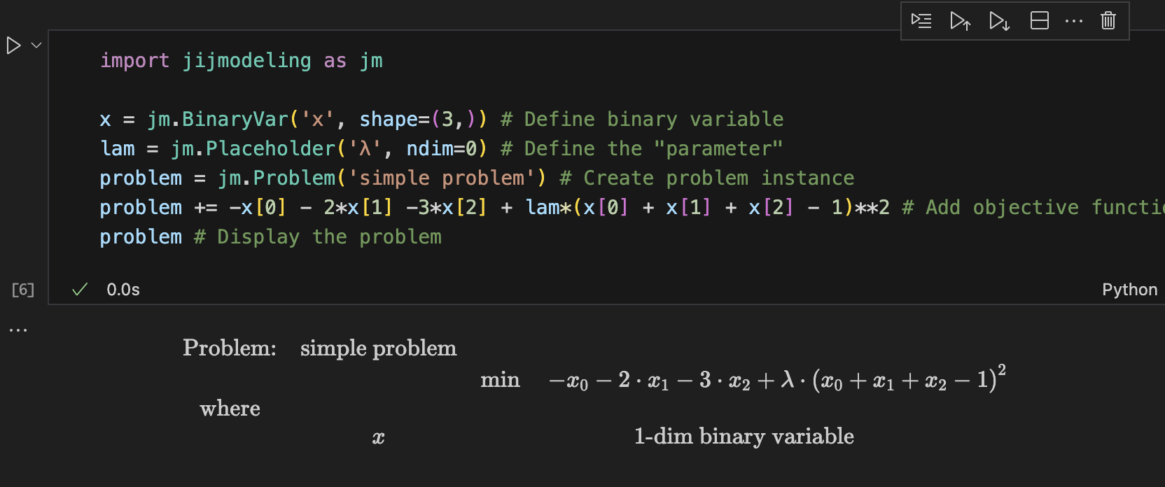
Let us now check the above phenomena by solving the problem with JijZept. Using JijModeling, the problem can be implemented as

import jijmodeling as jm

x = jm.BinaryVar('x', shape=(3,)) # Define binary variable
lam = jm.Placeholder('λ', ndim=0) # Define the "parameter"
problem = jm.Problem('simple problem') # Create problem instance
problem += -x[0] - 2*x[1] -3*x[2] + lam*(x[0] + x[1] + x[2] - 1)**2 # Add objective function
problem # Display the problem

Using the Jupyter Notebook environment, one can see the following mathematical expression of the problem.

Then, we solve the problem for $\lambda=0.0, 2.0, 3.0,\;{\rm and}\;50.0$ by JijSASampler, and check the frequency of obtained solutions for each $\lambda$.

import jijzept as jz
import matplotlib.pyplot as plt

# Prepare SASampler
sampler = jz.JijSASampler(config='*** your config.toml path ***')

# Define num_reads, the number of trials to solve.
num_reads=100

# Define λ list to solve
lam_list=[0, 2, 3, 50]

# Define function to draw th frequency graph
def plot_bars(sampleset, lam):
    counter = {0:0, 1:0, 2:0, 3:0, 4:0, 5:0, 6:0, 7:0}
    for sample in sampleset:
        solution = sample.to_dense()['x']
        state_number = 4*solution[0] + 2*solution[1] + solution[2]
        counter[state_number] += 1
    for key, val in counter.items():
        if key in [1,2,4]: # Feasible colored blue 
            plt.bar(key ,val,color='blue')
        else: # Infeasible colored red
            plt.bar(key ,val,color='red')
    plt.xlim(-0.5, 7.5)
    plt.ylim(0,num_reads)
    plt.xlabel('State number', fontsize=12)
    plt.ylabel('Count', fontsize=12)
    plt.title(f'λ={lam}')
    plt.show()

# Solve by JijZept
for lam in lam_list:
    response = sampler.sample_model(problem, {'λ': lam}, num_reads=num_reads)
    sampleset = response.get_sampleset()
    plot_bars(sampleset, lam)

Executing this code, one can obtain the result like this.

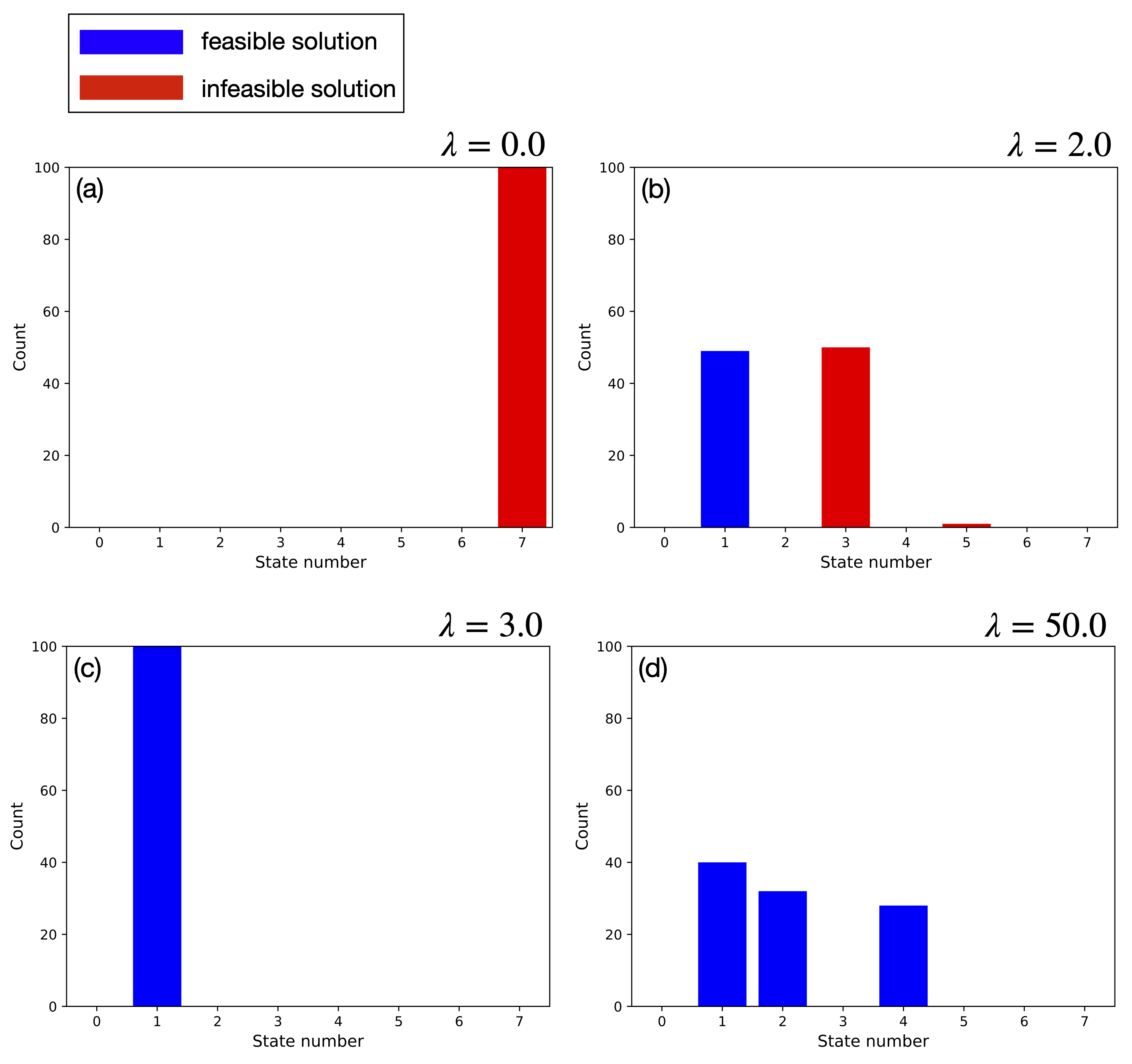Figure 2: Frequency of obtained solutions by JijSASampler for (a) $\lambda=0.0$, (b) $\lambda=2.0$, (c) $\lambda=3.0$, and (d) $\lambda=50.0$.

One can see that Fig. 2 is consistent with the previous discussion. When $\lambda=0.0$, the optimal solution for Eq. (2) corresponds to the state number 7, $(x_0,x_1,x_2)=(1,1,1)$, and all the solutions are the state number 7 [Fig. 2(a)]. While for $\lambda=2.0$, both $(0,0,1)$ and $(0,1,1)$, which corresponds to the state number 1 and 3, respectively, are optimal. Actually, the ratio of the solutions by JijSASampler are almost the same [Fig. 2(b)]. In contrast for $\lambda=3.0$, we obtained the unique optimal solution, the stat number 1 [Fig. 2(c)]. In the case of $\lambda=50.0$, the optimal solution is the stat number 1. The solutions by JijSASampler however are state number 1, 2, and 4 at almost the same rate owing to too large $\lambda$.

What is the Optimal Value for Parameters?

Our purpose is to obtain feasible and optimal solutions. Then what is the optimal value for the parameter $\lambda$? Unfortunately, there is little things to say about this point, because the optimal value depends on many things like mathematical problems, the characteristics of solvers, other tuning parameters, and so on. In our case, values around $\lambda=3$ are reasonable since the energy landscape is almost convex. See Fig. 3 below.

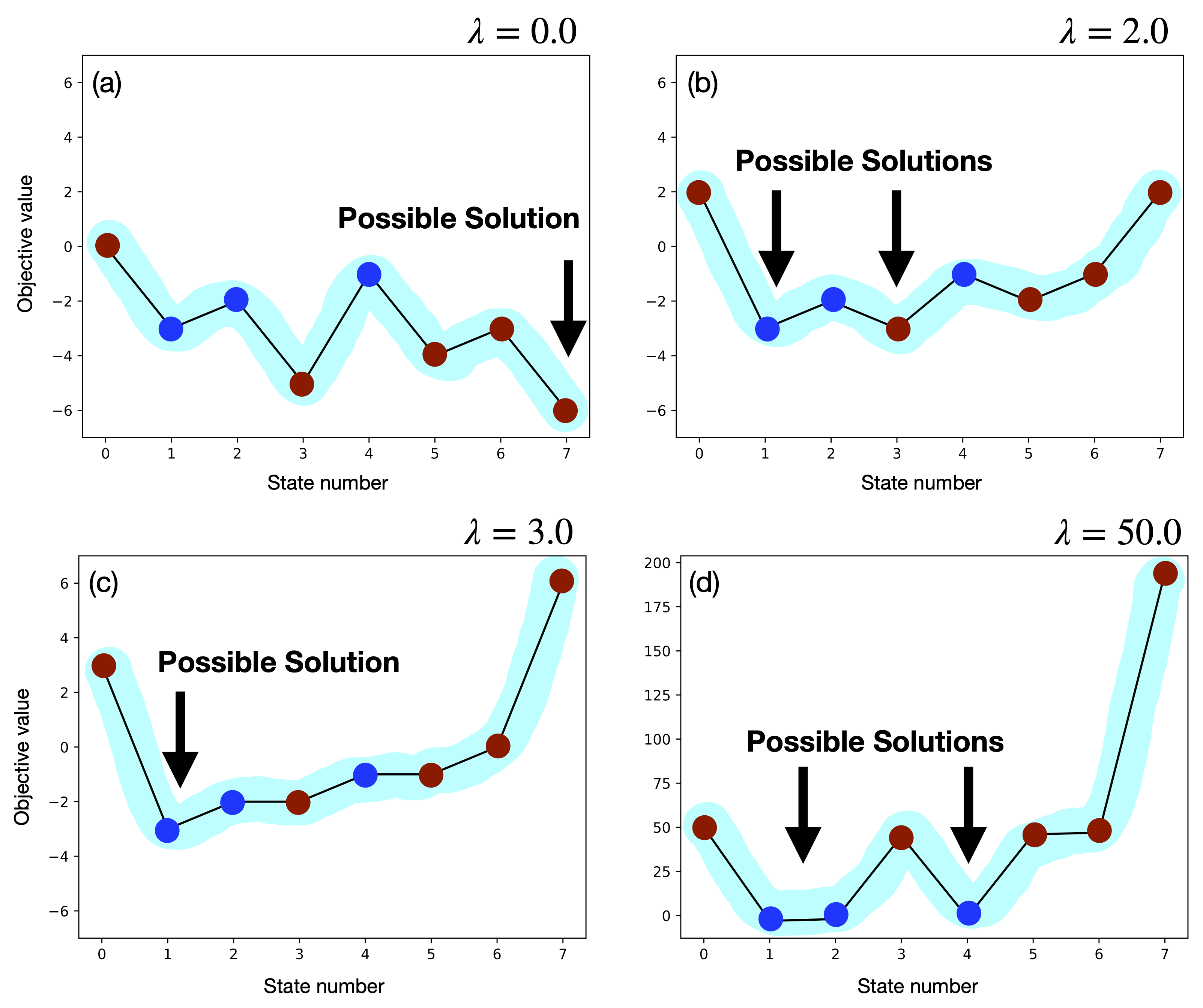Figure 3: Coarse-grained energy landscape (blue line) for (a) $\lambda=0.0$, (b) $\lambda=2.0$, (c) $\lambda=3.0$, and (d) $\lambda=50.0$.

In Fig. 3(a)-(d), we draw coarse-grained energy landscape roughly (blue line), and only the case for $\lambda=3.0$ is almost (but not exactly) convex and the optimal solution is feasible, leading to most solutions by Ising solvers being feasible and optimal. Actually all the solutions by JijSASampler are feasible and optimal [Fig. 2(c)]. Thus, we conclude that the optimal value for the parameter $\lambda$ is the value at which coarse-grained energy landscape is almost convex. Then, how do we find this optimal value? In general, it is difficult to determine $\lambda$, since it depends on many things as mentioned previously. We recommend that one should use the parameter search feature in JijZept to avoid difficulty of finding optimal value $\lambda$.

Parameter Search in JijZept

The solvers in JijZept have the parameter search feature, which can avoid difficulties of finding optimal parameters for constraint conditions. In this section, we show hot to use the parameter search of JijZept with a simple and well-known problem, the traveling salesman problem.

Traveling Salesman Problem

The traveling salesman problem (TSP) is one of a well-known problem as an example of mathematical optimization problems. There are some way to formulate the TSP. See this tutorial for the detail of the TSP. We here use the following mathematical expression as two-dimensional TSP.

import jijmodeling as jm

# Define variables
d = jm.Placeholder('d', ndim=2)
N = d.len_at(0, latex='N')
x = jm.BinaryVar('x', shape=(N, N))
i = jm.Element('i', belong_to=(0, N))
j = jm.Element('j', belong_to=(0, N))
t = jm.Element('t', belong_to=(0, N))

# Set problem
problem = jm.Problem('TSP')
problem += jm.sum([i, j], d[i, j] * jm.sum(t, x[i, t]*x[j, (t+1) % N]))
problem += jm.Constraint('one-city', x[:, t].sum() == 1, forall=t)
problem += jm.Constraint('one-time', x[i, :].sum() == 1, forall=i)

# Display mathematical expression
problem

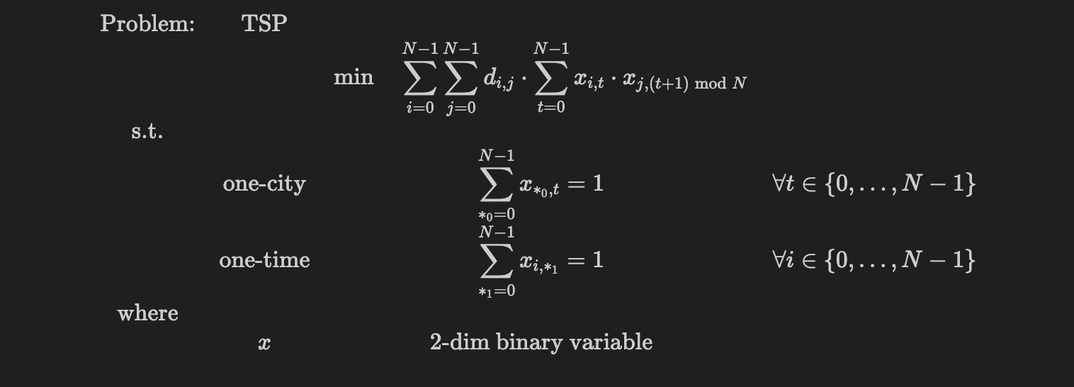
Here, $d_{i,j}=d_{j,i}>0$ is the distance between the cities, $N$ is the number of the cities, and $x_{i,t}$ is the decision variable. This problem has $2N$ constraint conditions. By using JijZept, the optimal parameters for these constraint conditions are automatically searched and there is no need to make effort to find the optimal values. Let us check this by executing the following code with using $N=30$ and random instance data for $d_{i,j}$.

import numpy as np
import jijzept as jz
import matplotlib.pyplot as plt

def tsp_distance(N: int):
    x, y = np.random.uniform(0, 1, (2, N))
    XX, YY = np.meshgrid(x, y)
    distance = np.sqrt((XX - XX.T)**2 + (YY - YY.T)**2)
    return distance, (x, y)


# Define the number of cities
num_cities = 30
distance, (x_pos, y_pos) = tsp_distance(N=num_cities)

# Setup SASampler
sampler = jz.JijSASampler(config='*** your config.toml path ***')

# Calculate by JijSASampler
response = sampler.sample_model(problem, {'d': distance}, search=True)
sampleset = response.get_sampleset()

# Extract feasible solution
feasible = sampleset.feasibles()

# Plot constraint violations for each parameter search step
plt.plot(
    [sample.eval.constraints['one-city'].total_violation for sample in sampleset],
    marker='o',
    label='one-city'
)
plt.plot(
    [sample.eval.constraints['one-time'].total_violation for sample in sampleset],
    marker='o',
    label='one-time'
)
plt.xlabel('Steps')
plt.ylabel('Constraint violations')
plt.title(f'The number of feasible solutions={len(feasible)}')
plt.legend()
plt.show()

# Plot histogram for objective values of feasible solutions
plt.hist([sample.eval.objective for sample in sampleset])
plt.xlabel('Objective value')
plt.ylabel('Count')
plt.title('Histogram for objective values of feasible solutions')
plt.show()

Figure 4: (a) History of constraint violations at each parameter search step. (b) Histogram of objective value by feasible solutions.

One can obtain the results like the above. Figure 4(a) shows history of constraint violations at each parameter search step, where constraint violations are defined as

$${\rm one-city:\;\;\;}\sum^{N-1}_{t=0}\left\|\sum^{N-1}_{i=0}x_{i,t}-1\right\|,{\rm with\;the\;solution}\;x_{i,t},$$$${\rm one-time:\;\;\;}\sum^{N-1}_{i=0}\left\|\sum^{N-1}_{t=0}x_{i,t}-1\right\|,{\rm with\;the\;solution}\;x_{i,t}.$$

In this case, both constraint violations take zero at the same time in the parameter search steps, which means we obtain the feasible solutions. At this time, we obtain two feasible solutions with the objective values around 8.5 and 9.65. See Fig. 4(b). One can modify settings of the parameter search. For example, setting num_search=20 executes the parameter search 20 steps, setting num_reads=10 execute calculations 10 times at each parameter search steps, and multipliers={'one-city': 1.0, 'one-time': 1.0} sets the initial values of the parameter search. See the class reference of sample_model for the details.