Samplers
JijZept has many kinds of solvers for mathematical models of optimization problems. We here show the detailed usage of these solvers. First, we explain common features of these solvers, then we describe how to read calculation status, error messages, and so on. Finally, we briefly demonstrate some solvers with specific features.
Basic Usage
In this section, we explain basic and common usage of JijZept, which has following samplers to solver optimization problems.
JijSASampler: Simulated annealing sampler implemented by Jij.JijSQASampler: Simulated quantum annealing sampler implemented by Jij.JijSolver: Local search solver implemented by Jij.JijDA4Sampler: Sampler using Fujitsu Digital Annealer version 4.JijLeapHybridCQMSampler: Sampler using Leap’s Hybrid Solvers.JijFixstarsAmplifySampler: Sampler using Fixstars Amplify.
Set Up Samplers
The above sampler classes are provided in JijZept as a python module. One needs API key of JijZept to initialize these samplers. For example, the following code sets up jz.JijSASampler.
import jijzept as jz
sampler = jz.JijSASampler(token='*** your API key ***', url='https://api.jijzept.com')
One can also use config.toml file for the initialization.
import jijzept as jz
sampler = jz.JijSASampler(config='*** your config.toml path ***')
Here, the contents of config.toml file should be like as follows.
[default]
url = "https://api.m.jijzept.com/"
token = "*** your API key ***"
Third Party Solvers
Three solvers, JijDA4Sampler, JijLeapHybridCQMSampler, and JijFixstarsAmplifySampler need extra authentication information. One must need to contract and receive API key or something about each solver. For example, JijDA4Sampler can be initialized as follows.
import jijzept as jz
sampler = jz.JijDA4Sampler(
    token='*** your API key ***',
    url='https://api.jijzept.com',
    da4_token='*** your DA4 token ***'
)
Or, one can also use
import jijzept as jz
sampler = jz.JijDA4Sampler(
    config='*** your config.toml path ***',
    da4_token='*** your DA4 token ***'
)
These solvers are named third party solvers.
Sampling Method
Now, the above noted samplers have the method called sample_model. The method is solver for any mathematical model using JijModeling.
To learn how to use sample_model, let's start by construct a mathematical model using JijModeling. Please see the documentation for the detailed usage. Here, we use the simple example.
import jijmodeling as jm
d = jm.Placeholder('d', ndim=1) # Define variable d
d.len_at(0, latex='N') # Set latex expression of the length of d
x = jm.BinaryVar('x', shape=(d.shape[0],)) # Define binary variable
i = jm.Element('i', belong_to=(0, d.shape[0])) # Define dummy index in summation
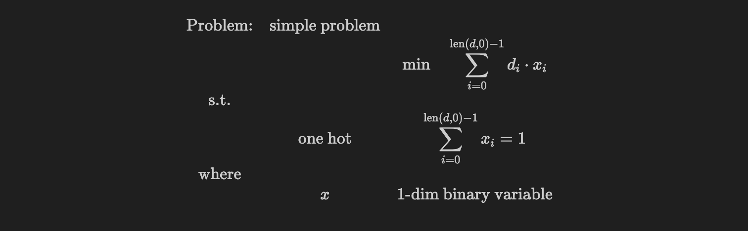
problem = jm.Problem('simple problem') # Create problem instance
problem += jm.sum(i, d[i]*x[i]) # Add objective function
problem += jm.Constraint('one hot', jm.sum(i, x[i]) == 1) # Add constraint condition
problem # Display the problem
Using the Jupyter Notebook environment, one can see the mathematical expression.
Then, we solve the problem by sample_model, which has the basic parameters.
| Parameters | Description |
|---|---|
feed_dict | The instance data to the placeholders. |
multipliers | The multipliers for penalty terms, derived from constraint conditions. If the parameter search is enabled, this value used as initial values. |
search | If True, the parameter search will be enabled, which tries to find better values of multipliers for penalty terms from constraint conditions. |
num_search | The number of parameter search iteration. This option works when the parameter search is enabled. |
sample_model has more tuning parameters depending on the samplers. See the class reference. Now, let us solve the problem by sample_model.
from jijzept import JijSASampler

# Instance data for d, the key is the name of placeholder and the value is actual values
instance_data = {'d': [1.0, 0.1, -2.0, 1.0]}

# Set up sampler
sampler = JijSASampler(config='*** your config.toml path ***')

# Solve by sample_model
response = sampler.sample_model(
    problem,
    instance_data,
    multipliers={'one-hot': 1.0}, # The key is the name of constraint conditions.
    search=True,
    num_search=10
)
One can see the feasible solutions like this.
# Get feasible solutions.
sampleset = response.get_sampleset().feasibles()

# Display the solutions and the objective values.
for sample in sampleset.feasibles():
    print(f"solution: {sample.to_dense()}, objective: {sample.eval.objective}")
Please check if the optimal and feasible solution with the objective value -2.0 are obtained. If you want to know how the solution information is stored, see What is SampleSet.
Parameters Class
For each solver, there is an associated Parameters class.
To configure the solver, instantiate the Parameters class for your solver and pass the instance to the parameters argument of sample_* method.
Here's an example with the JijSASampler.
import jijmodeling as jm
from jijzept import JijSASampler
from jijzept.sampler import JijSAParameters

d = jm.Placeholder('d', ndim=1) # Define variable d
d.len_at(0, latex='N') # Set latex expression of the length of d
x = jm.BinaryVar('x', shape=(d.shape[0],)) # Define binary variable
i = jm.Element('i', belong_to=(0, d.shape[0])) # Define dummy index in summation
problem = jm.Problem('simple problem') # Create problem instance
problem += jm.sum(i, d[i]*x[i]) # Add objective function
problem += jm.Constraint('one hot', jm.sum(i, x[i]) == 1) # Add constraint condition

# Instance data for d, the key is the name of placeholder and the value is actual values
instance_data = {'d': [1.0, 0.1, -2.0, 1.0]}

sampler = JijSASampler(config='*** your config.toml path ***') # Create sampler instance
parameters = JijSAParameters(num_sweeps=2000, num_reads=10) # Create parameters instance

# Solve by sample_model
response = sampler.sample_model(
    problem,
    instance_data,
    multipliers={'one-hot': 1.0}, # The key is the name of constraint conditions.
    search=True,
    num_search=10,
    parameters=parameters, # Set parameters
)
In this case, num_sweeps sets the number of Monte-Carlo steps, and num_reads sets the number of samples per search.
Available Options
sample_model provide two options, sync and max_wait_time.
Sync Option
With the default settings, after throwing a problem to JijZept, the process blocks until the answer is returned, which can be inconvenient when solving process takes a long time. Setting the parameter to sync=False, which is the asynchronous mode, will return the control immediately after the problem is thrown to JijZept.
response = sampler.sample_model(
    problem,
    instance_data,
    multipliers={'one-hot': 1.0},
    search=True,
    num_search=10,
    sync=False, # Set to asynchronous mode
)
At this mode, one can obtain the result by get_result after the solving process is completed.
sample_set.get_result()
You can also retrieve the solution from stored solution_ids.
sampler = jz.JijSASampler(config="*** your config.toml path ***")
ids = []
for i in range(10):
    response = sampler.sample_model(problem, instance_data, search=True, sync=False)
    ids.append(response.solution_id)

# Get the first result.
response.get_result(solution_id=ids[0])
Max Wait Time Configuration
The max_wait_time option allows you to set a time limit on how long the solvers will run. If the computation time is exceeded, FAILED will be returned. The following example sets a time limit as 10 seconds.
response = sampler.sample_model(
    problem,
    instance_data,
    multipliers={'one-hot': 1.0},
    search=True,
    num_search=10,
    max_wait_time=10 # seconds
)
Note that the default value of max_wait_time is 60 (1 minute).
Note: Before version 1.14.1,
max_wait_timewas namedtimeout, but now the use oftimeoutis deprecated. To bring your code up to date with the latest standards, replace thetimeoutargument with themax_wait_timeargument.
Solving Status and Error Messages
The return value of the samplers, the above mentioned sample_set, stores calculation status of JijZept, which are the following types.
| Status | Description |
|---|---|
SUCCESS | Calculation was successfully completed. |
PENDING | A problem has been submitted and has not yet been passed to solvers. |
RUNNING | A problem has been submitted and passed to solvers. |
FAILED | Failed to solver problems. See sample_set.error_message for the details. |
UNKNOWNERROR | Failed to solver problems due to unexpected causes. |
If the calculation status is FAILED, one can see the error messages in sample_set.error_message. We here show the example by setting short calculation time, max_wait_time=0.01.
response = sampler.sample_model(
    problem,
    instance_data,
    multipliers={'one-hot': 1.0},
    search=True,
    num_search=10,
    max_wait_time=0.01 # seconds
)

print(response.status) # Show status
print(response.error_message) # Show error messages
We expect that the following output is showed.

Solvers with Specific Features
Some solvers in JijZept has specific features, satisfying some types of constraint conditions. In this section, we briefly explain these solvers.
JijDA4Sampler
JijDA4Sampler can find the feasible solutions for one-way and two-way one-hot constraint conditions, where one-way one-hot constraint conditions mean just one-hot ones compared to two-way one-hot ones, and two-way one-hot ones are like the constraint conditions appeared in the traveling salesman problem (TSP).
Let us here use the TSP as an example of the problem with two-way one-hot constraint conditions.
import jijmodeling as jm
# Define variables
d = jm.Placeholder('d', ndim=2)
N = d.len_at(0, latex='N')
x = jm.BinaryVar('x', shape=(N, N))
i = jm.Element('i', belong_to=(0, N))
j = jm.Element('j', belong_to=(0, N))
t = jm.Element('t', belong_to=(0, N))
# Set problem
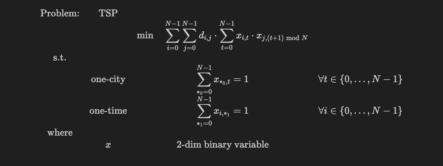
problem = jm.Problem('TSP')
problem += jm.sum([i, j], d[i, j] * jm.sum(t, x[i, t]*x[j, (t+1) % N]))
problem += jm.Constraint('one-city', x[:, t].sum() == 1, forall=t)
problem += jm.Constraint('one-time', x[i, :].sum() == 1, forall=i)
# Display mathematical expression
problem
Then, we solve the problem with two-dimensional random instance by JijDA4Sampler. There is no need to take some efforts to treat the constraint conditions. JijDA4Sampler extracts one-way and two-way one-hot constraint conditions and find feasible solutions.
import numpy as np
from jijzept import JijDA4Sampler

def tsp_distance(N: int):
    x, y = np.random.uniform(0, 1, (2, N))
    XX, YY = np.meshgrid(x, y)
    distance = np.sqrt((XX - XX.T)**2 + (YY - YY.T)**2)
    return distance, (x, y)


# Define the number of cities
num_cities = 10
distance, (x_pos, y_pos) = tsp_distance(N=num_cities)

# Setup SASampler
sampler = JijDA4Sampler(
    config='*** your config.toml path ***',
    da4_token='*** your DA4 token ***'
)
# Calculate by JijSASampler
response = sampler.sample_model(problem, {'d': distance})
sampleset = response.get_sampleset()

for sample in sampleset:
    print(f'objective: {sample.eval.objective}')
    print(f'violation of one-city: {sample.eval.constraints["one-city"].total_violation}')
    print(f'violation of one-time: {sample.eval.constraints["one-time"].total_violation}')
Please check the constraint violations are zero.
Return Value of Samplers
The SampleSet described below will be deprecated at the end of April 2024. Please see What is SampleSet for a description of the new SampleSet.
In this section, we explain the return value of samplers in JijZept, which stores various information about solutions and is provided as jijmodeling.SampleSet class. It is better to use SampleSet.Record and SampleSet.Evaluation to analyze the quality of the solution, e.g., the value of the objective function, the degree of constraint violation, etc.
In the following, we use the mathematical model as follows and solve it by JijSASampler.
import jijmodeling as jm
N = jm.Placeholder('N')
a = jm.Placeholder('a', ndim=2)
x = jm.BinaryVar('x', shape=(N,N))
i = jm.Element('i', belong_to=(0, N))
j = jm.Element('j', belong_to=(0, N))
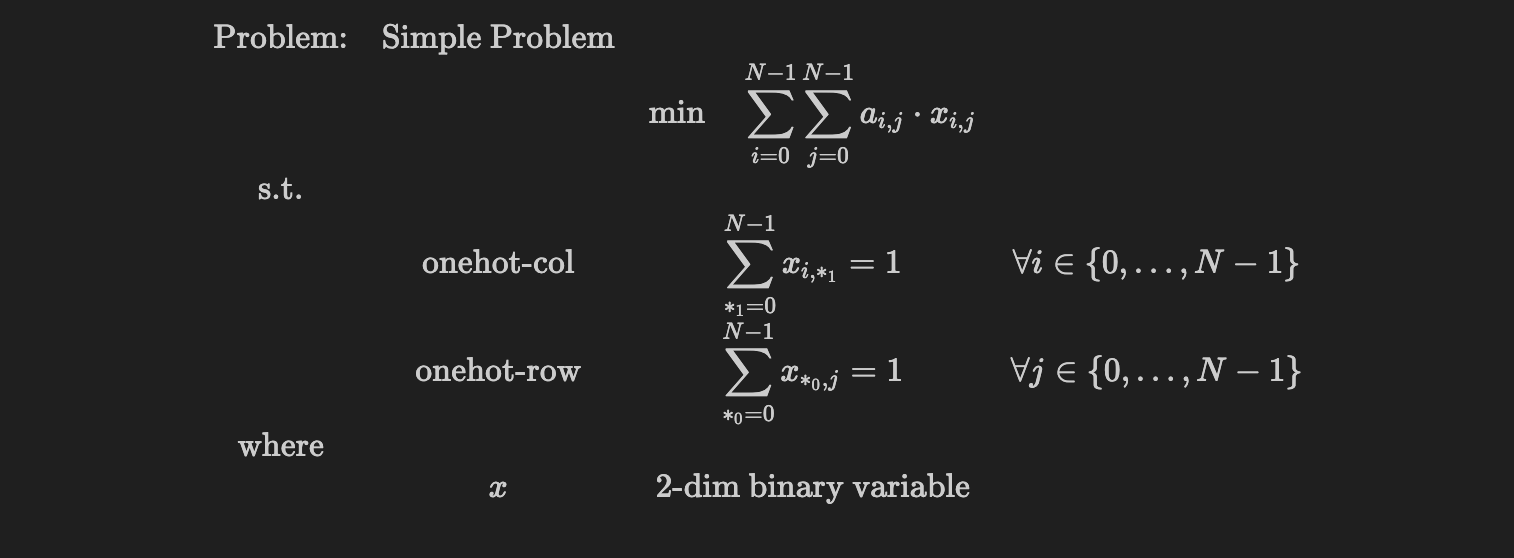
problem = jm.Problem('Simple Problem')
problem += jm.sum([i, j], a[i, j]*x[i, j])
problem += jm.Constraint('onehot-row', x[:, j].sum() == 1, forall=j)
problem += jm.Constraint('onehot-col', x[i, :].sum() == 1, forall=i)
problem
We use the parameter search by setting search=True to obtain feasible solutions.
instance_data={'N': 3, 'a': [[1, 2, 3], [4, 5, 6], [7, 8, 9]]}
sampler = jz.JijSASampler(config='config.toml')
sample_set = sampler.sample_model(problem, instance_data, search=True, num_search=5)
Here, sample_set object stores 5 solutions since the parameter search is executed 5 times by num_search=5.
Record
SampleSet.Record mainly stores the solutions and the occurrences of the solutions. The solutions are stored in sparse representation by default and is represented by tuple non-zero indices, non-zero values, shape of decision variables. We first look the solutions stored in Record.solution.
sample_set.record.solution
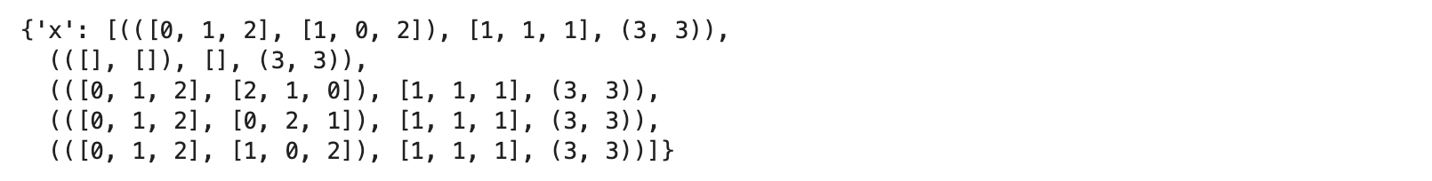
Here, the key x is the name of the decision variable jm.Binary('x', shape=(N,)) and the value of the list represents the solutions in sparse representation. For example, the first element of the list is (([0, 1, 2], [1, 0, 2]), [1, 1, 1], (3, 3)), and the first element of this tuple ([0, 1, 2], [1, 0, 2]) represents the non-zero indices of the decision variable x. To be more specific, since the decision variable is two-dimensional list, ([0, 1, 2], [1, 0, 2]) means only x[0][1], x[1][0], and x[2][2] take non-zero values. Then, [1, 1, 1] is the none-zero value and is here 1. The last element (3, 3) represents the shape of the decision variable x, where x consists of two-dimensional list. Let us check this by dense representation.
sample_set.to_dense().record.solution
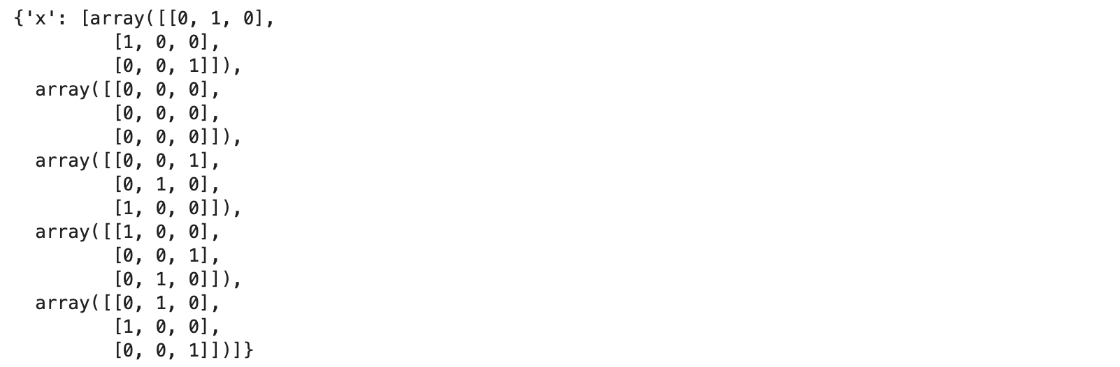
Actually, one can see that only x[0][1], x[1][0], and x[2][2] take 1 for the first solution.
Then, we explain Record.num_occurrences, which shows the number of occurrences about the solutions. We here obtain 5 different solutions. Thus,
sample_set.record.num_occurrences
shows [1, 1, 1, 1, 1], since all solutions obtained here are different from each other.
Evaluation
SampleSet.Evaluation mainly stores information about evaluating solutions, including the energy, the value of objective function, and the degree of constraint violations.
objective
Evaluation.objective shows the values of the objective function for the solutions. We here obtain the 5 solutions and one can easily see that the the values of the objective function is 15, 0, 15, 15, and 15. Thus, Evaluation.objective shows as follows.
sample_set.evaluation.objective

constraint_violations
Evaluation.constraint_violations calculates how much the constraint conditions are violated. In general, if a constraint condition for a binary variable
is added, constraint_violations calculate
with taking the summation of forall indices.
To be more specific for this case, constraint_violations is defined as follows.
For satisfying the constraint condition "onehot-row", only one binary variable take 1 for each row. The second solution however takes all zeros, and thus, constraint_violations takes 1 for each row leading to 3 in total. The same applies to the constraint condition "onehot-col".
Let us check the values.
sample_set.evaluation.constraint_violations

We here obtain 5 solutions and only the second one breaks the constraint conditions. Thus, constraint_violations for other solutions takes zero.
Filtering Solutions
jijmodeling.SampleSet has some convenient methods to extract the solutions with specific features.
Infeasible Solutions
SampleSet.infeasible() method extracts the infeasible solutions, which break at least one constraint condition.
sample_set.infeasible()
Feasible Solutions
SampleSet.feasible() method extracts the feasible solutions, which satisfy all the constraint conditions.
sample_set.feasible()
Lowest Solutions
SampleSet.lowest() method extracts the solutions taking the minimum value of the objective functions among the feasible solutions. If there are multiple minimum values, lowest() method returns all these solutions.
sample_set.lowest()