Simulated Annealing

Here, we introduce the simulated annealing (SA) [1] to solve the unconstraint optimization problems with JijZept. This method is based on the physical process of annealing the iron, and one can obtain a certain level of solutions.

What is the Simulated Annealing?

SA is a method for solving combinatorial optimization problems and is one of the meta-heuristics, which is a general term for heuristics. SA can be applied generally to many combinatorial optimization problems with no constraint conditions. The problems with some kind of constraint conditions can also be solved by SA using the penalty methods. The general process to solve the problems by SA is repeating the following two steps.

• Obtain a new solution according to the previous computation steps
• Evaluate the new solution and store the information to search for a new solution in the next computation step.

Let us consider a more concrete example. The solution to a combinatorial optimization problem is represented as a bit sequence of $\{0, 1\}$ such as $(0, 0, 1, 0, \dots)$ or $(1, 1, 1, 0, \dots)$. These bit sequences are called the states. The set of the states that are "close" in some kind of meaning to a certain bit sequence $\boldsymbol{x}$ is called a neighborhood $N(\boldsymbol{x})$ of $\boldsymbol{x}$. The computation steps of SA can be represented in more detail as follows.

• Select a state $\boldsymbol{x}'$ randomly from the neighborhood $N(\boldsymbol{x})$ of the state $\boldsymbol{x}$ in the previous step.
• Update the state $\boldsymbol{x}'$ from $\boldsymbol{x}$ with probability $P(E(\boldsymbol{x}), E(\boldsymbol{x}'), T)$.

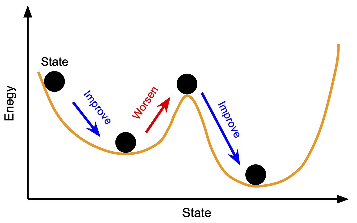
Here, $E(\boldsymbol{x})$ represents the energy and corresponds to the value of the objective function in the mathematical model of the combinatorial optimization problem. $T$ is a non-negative parameter, which can be considered as the temperature. One must determine the value of $T$ for each calculation step in advance. Usually, the temperature $T$ is decreased with each calculation step. This is expected to cause the state $\boldsymbol{x}$ to change frequently when the temperature is high, but as the temperature decreases, the state $\boldsymbol{x}$ is expected to converge to the globally optimal solution. This is why it is called simulated "annealing. The figure below shows how the state improves as the calculation steps progress.

Now, in the above algorithm, we have to determine the way to construct the neighborhood $N(\boldsymbol{x})$ from $\boldsymbol{x}$ and the way to set the transition probability $P(E(\boldsymbol{x}), E(\boldsymbol{x}'), T)$ for executing the SA. The simple way to set up a neighborhood is to define $N(\boldsymbol{x})$ as "the set of states that can be reached by a single bit flip from the state $\boldsymbol{x}$". Algorithms using this neighborhood definition are generally called single-spin flips. As for the transition probability $P(E(\boldsymbol{x}), E(\boldsymbol{x}'), T)$, a relatively good solution can be obtained by using the following setting.

$$P(E(\boldsymbol{x}), E(\boldsymbol{x}'), T) = \left\{ \begin{array}{ll} e^{-(E(\boldsymbol{x}') - E(\boldsymbol{x})) /T} & (E(\boldsymbol{x}') > E(\boldsymbol{x})) \\ 1 & (E(\boldsymbol{x}') \leq E(\boldsymbol{x})) \end{array} \right.\tag{1}$$

Using this setting of the transition probability is called the Metropolis method. The figure below plots the probability $P(E(\boldsymbol{x}), E(\boldsymbol{x}'), T)$ set by the above equation (1).

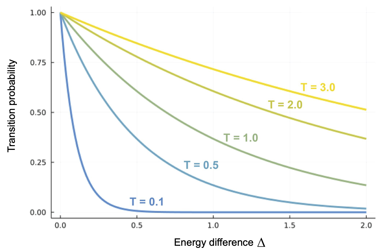
Here, the x-axis is the energy difference between the states $\Delta=E(\boldsymbol{x}') - E(\boldsymbol{x})$. Note that the transition probability is always 1 in the case of $\Delta \leq 0$. When the temperature $T$ is high, a random update of the state is more likely to occur since the transition probability is large even when $\Delta>0$. This prevents the state $\boldsymbol{x}$ from remaining in the locally optimal solution. As the calculation progresses and the temperature decreases, the transition probability becomes smaller for $\Delta>0$. This results in the state being updated only when the energy is reduced. This is expected to cause the state $\boldsymbol{x}$ to converge to the globally optimal solution.

Characteristics of SA

The SA has the following advantages and is often used to solve combinatorial optimization problems.

• The SA can prevent the state from being trapped in locally optimal solutions by using thermal fluctuations.
• The algorithm does not depend on the details of objective functions, and thus it can be applied to a wide range of combinatorial optimization problems.
• It is easy to understand and implement the algorithm of the SA.

In contrast, the SA has the following disadvantage.

• Obtaining the exact optimal solution needs a long calculation time or may be impossible in the reasonable calculation time.
• It is difficult to handle constraint conditions directly. They must be handled indirectly by using penalty methods or something.
• Proper scheduling for temperature $T$ depends on the mathematical problems and needs some effort.

The SA is useful for obtaining solutions in practical computation time that may not be optimal, but are reasonably good.

Calculation with JijZept

In this section, we explain how to obtain solutions by the SA using JijZept. First, you must finish setup of JijZept and get API key. Then you can prepare JijSASampler in JijZept, which solve the problem by using the SA.

import jijzept as jz

# Setup SA Sampler
sampler = jz.JijSASampler(token='*** your API key ***', url='https://api.jijzept.com')

Here, we explain how to solve mathematical problems using JijModeling. Please see the documentation for how to use JijModeling. We use the following optimization problem with the constraint condition as a simple example.

$${\rm min} -\sum^{N-1}_{i=0}d_i x_i\\ {\rm subject\;to}\;\;\;\sum^{N-1}_{i=0}x_i=1\\ x_i\in\{0,1\}$$

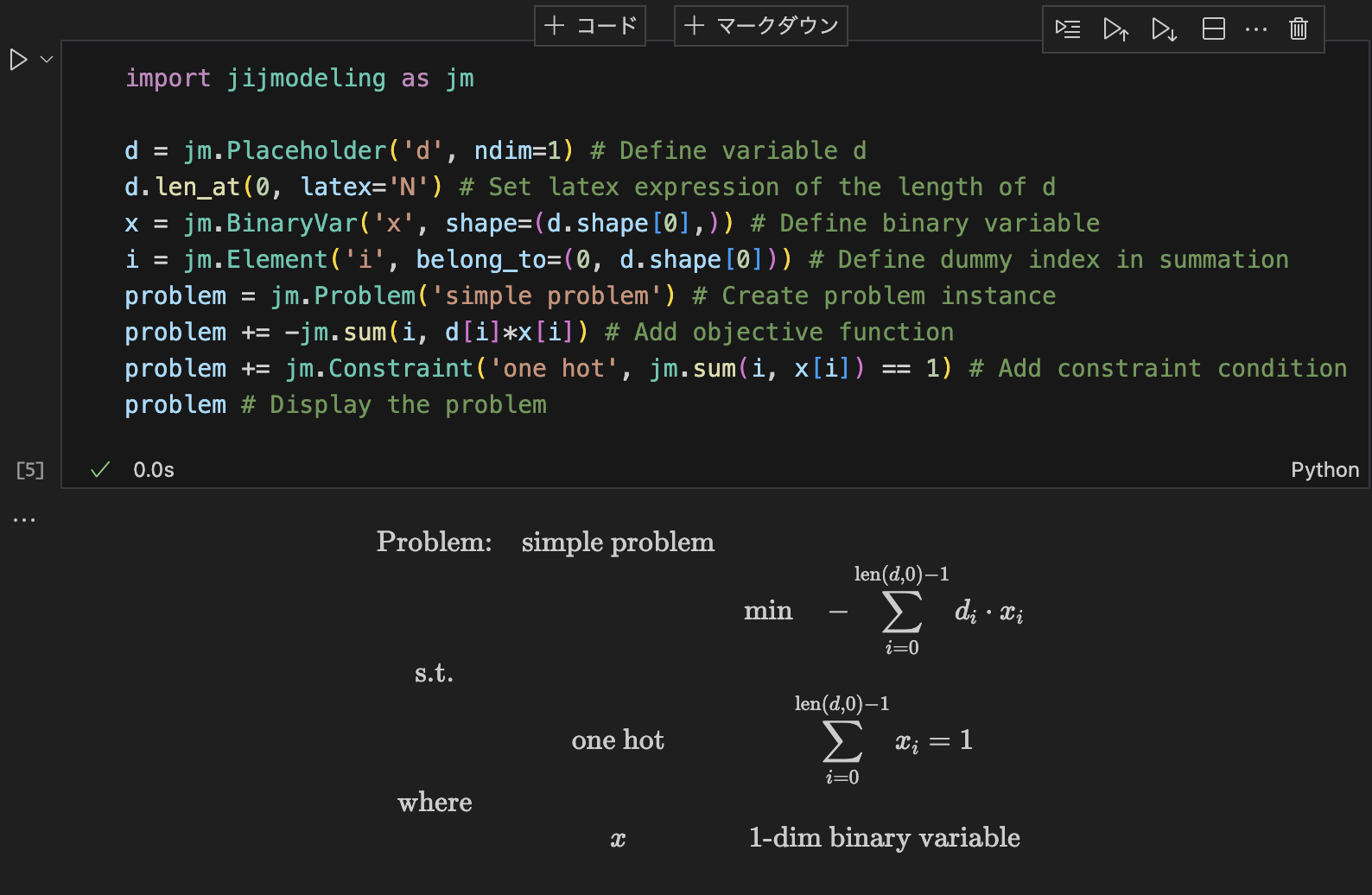
This problem can be implemented by JijModeling as follows.

import jijmodeling as jm

d = jm.Placeholder('d', ndim=1) # Define variable d
d.len_at(0, latex='N') # Set latex expression of the length of d
x = jm.BinaryVar('x', shape=(d.shape[0],)) # Define binary variable
i = jm.Element('i', belong_to=(0, d.shape[0])) # Define dummy index in summation
problem = jm.Problem('simple problem') # Create problem instance
problem += -jm.sum(i, d[i]*x[i]) # Add objective function
problem += jm.Constraint('one hot', jm.sum(i, x[i]) == 1) # Add constraint condition
problem # Display the problem

Using the Jupyter Notebook environment, one can see the following mathematical expression of the problem.

Then, we consider the exact optimal solution. If $d_i>0$ for all $i=0,1,\ldots,N-1$, solving the above problem is equal to finding the maximum value of $d_i$. Thus, considering the instance value $d=(1,2,3,2,1)$, the exact optimal solution is $\boldsymbol{x}=(0,0,1,0,0)$ with the energy -3.0. Now we check the solution obtained by JijZept.

instance_data = {'d': [1,2,3,2,1]} # The actual value of d

# search=True: Use parameter search, num_search: The number of trials for parameter search
response = sampler.sample_model(problem, instance_data, search=True, num_search=5)
# Get solutions
sampleset = response.get_sampleset()
for sample in sampleset:
    # Display the solutions and the objective values
    print(f'solution:{sample.to_dense()}, objective: {sample.eval.objective}')

For example, suppose the output is as follows:

solution:{'x': array([0., 0., 1., 0., 0.])}, objective: -3.0
solution:{'x': array([1., 1., 1., 1., 1.])}, objective: -9.0
solution:{'x': array([0., 0., 1., 0., 0.])}, objective: -3.0
solution:{'x': array([0., 0., 1., 0., 0.])}, objective: -3.0
solution:{'x': array([0., 0., 1., 0., 0.])}, objective: -3.0

In this case, the exact optimal solution $\boldsymbol{x}=(0,0,1,0,0)$ was obtained four times in the calculation.

Finally, we note that the above samplers have additional parameters to obtain better solutions. If you want to tune these parameters, see the class reference.

References

[1] S. Kirkpatrick, C. D. Gelatt, Jr., and M. P. Vecchi, Optimization by Simulated Annealing