Clique Problem

Here we show how to solve clique using JijZept and JijModeling. This problem is also mentioned in 2.3. Clique on Lucas, 2014, "Ising formulations of many NP problems".

What is Clique Problem?

This is a decision problem of whether or not a clique (complete graph) of size $K$ exists in a given graph.

Complete graphs

A complete graph is a graph whose two vertices are all adjacent to each other (not including loops or multiple edges). We show two examples below.

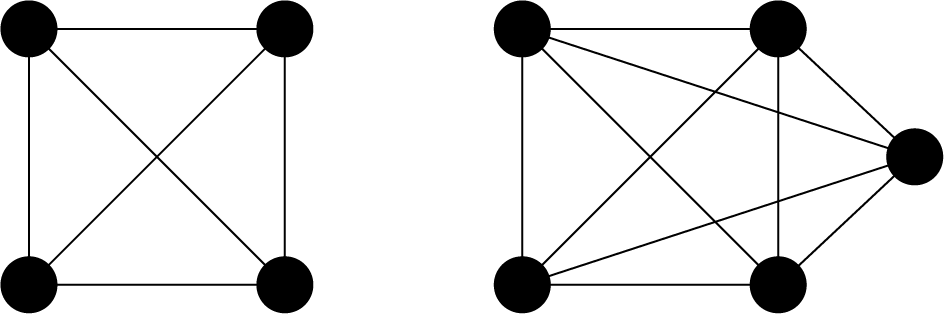
As mentioned above, a vertex in a complete graph is adjacent to all other vertices. A complete undirected graph $G = (V, E)$ has ${}_V C_2 = \frac{1}{2} V(V-1)$ edges, that is, the number of edges is equal to the number of combinations choosing two vertices from $V$.

Mathematical Model

First, we introduce binary variables $x_{v}$ which are 1 if vertex $v$ belongs to the subgraph and 0 otherwise.

Constraint 1: sum of $x_v$ must equal K

In this problem, each vertex $x_v$ either be 1 if vertex $v$ is selected as part of the subgraph, and 0 otherwise.

$$\sum_{v=0}^{V-1} x_{v} = K \tag{1}$$

Constraint 2: the subgraph must be complete

If the subgraph $G (W, E_W)$ where $E_W$ represents the subset of edges $E$ restricted to those connecting nodes within $W$, is complete, then the number of edges in this subgraph is given by $\frac{1}{2} W (W -1)$ from previous discussion. Knowing that the subgraph has $\sum_{(uv) \in E_W} x_{u} x_{v}$ edges, we set the constraint function as follows.

$$\sum_{(uv) \in E} x_{u} x_{v} = \frac{1}{2} K(K-1) \tag{2}$$

Modeling by JijModeling

Next, we show an implementation using JijModeling. We first define variables for the mathematical model described above.

import jijmodeling as jm

# define variables
V = jm.Placeholder('V')
E = jm.Placeholder('E', ndim=2)
K = jm.Placeholder('K')
x = jm.BinaryVar('x', shape=(V,))
u = jm.Element('u', (V))
e = jm.Element('e', E)

We use the same variables in the graph partitioning problem, and we add $K$ to that.

Constraint 1

We implement constraint Equation (1).

# set problem
problem = jm.Problem('Clique')
# set constraint: sum of $x_v$ must equal K
problem += jm.Constraint('constraint1', jm.sum(u, x[u])==K)

Constraint 2

Next, we implement constraint Equation (2).

# set constraint: the subgraph must be complete
problem += jm.Constraint('constraint2', jm.sum(e, x[e[0]]*x[e[1]])==1/2*K*(K-1))

Let's display the implemented mathematical model in Jupyter Notebook.

problem

$\begin{array}{cccc}\text{Problem:} & \text{Clique} & & \\& & \min \quad \displaystyle 0 & \\\text{{s.t.}} & & & \\ & \text{constraint1} & \displaystyle \sum_{u = 0}^{V - 1} x_{u} = K & \\ & \text{constraint2} & \displaystyle \sum_{e \in E} x_{e_{0}} \cdot x_{e_{1}} = 0.5 \cdot K \cdot \left(K - 1\right) & \\\text{{where}} & & & \\& x & 1\text{-dim binary variable}\\\end{array}$

Prepare an instance

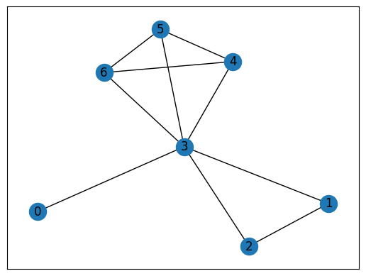
We prepare a graph by using Networkx, focusing on a scenario where the graph includes a complete subgraph of size $K=4$.

import networkx as nx

# set the number of random vertices
inst_V1 = 3
# create a random graph
inst_G1 = nx.gnp_random_graph(inst_V1, 0.2)

# set the size K
inst_K = 4
# create a complete graph with K vertices
inst_G2 = nx.complete_graph(inst_K)

# set the number of vertices
inst_V = inst_V1 + inst_K

# add the complete graph to the given graph
inst_G = nx.union(inst_G1, inst_G2, rename=('G-', 'K-'))

# connect each vertex of G1 to vertex 0 of G2
for i in range(inst_V1):
    inst_G.add_edge(f'G-{i}', 'K-0')

# relabel the nodes using normal numbers from 0
mapping = {node: i for i, node in enumerate(inst_G.nodes)}
inst_G = nx.relabel_nodes(inst_G, mapping)

# get information of edges
inst_E = [list(edge) for edge in inst_G.edges]

instance_data = {'V': inst_V, 'E': inst_E, 'K': inst_K}

This graph for clique problem is shown below.

import matplotlib.pyplot as plt

pos = nx.spring_layout(inst_G)
nx.draw_networkx(inst_G, pos, with_labels=True)

plt.show()

Solve by JijZept's SA

We solve this problem using JijZept JijSASampler. We also use the parameter search function by setting search=True.

import jijzept as jz

# set sampler
config_path = "config.toml"
sampler = jz.JijSASampler(config=config_path)
# solve problem
multipliers = {'constraint1': 0.5, "constraint2": 0.5}
response = sampler.sample_model(problem, instance_data, multipliers, num_reads=100, search=True)

Visualize solution

In the end, we extract the lowest energy solution from the feasible solutions and visualize it.

import numpy as np

# get sampleset
sampleset = response.get_sampleset()
# extract feasible samples
feasible_samples = sampleset.feasibles()
# get the solution
solution = feasible_samples[0].var_values["x"].values
# get the vertex numbers
vertices = [key[0] for key in solution]
print(vertices)
# set color list for visualization
cmap = plt.get_cmap("tab10")
# initialize vertex color list
node_colors = [cmap(0)] * instance_data["V"]
# set the vertex color list
for i in vertices:
    node_colors[i] = cmap(1)
# highlight the edge of clique
highlight_edges = [(u, v) for (u, v) in inst_G.edges() if u in vertices and v in vertices]
# make figure
nx.draw_networkx(inst_G, pos, node_color=node_colors, with_labels=True)
nx.draw_networkx_edges(inst_G, pos, edgelist=highlight_edges, edge_color='red')
plt.show()

[5, 4, 3, 6]

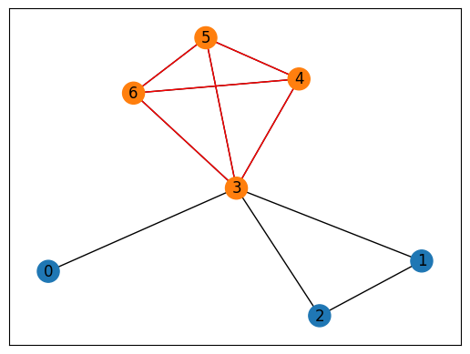
We obtain a feasible clique as shown above.

Lastly, we will introduce a trick to reduce the number of extra spins needed to encode a variable that can take $N$ values. By defining an integer $M$, where $2^M \leq N < 2^{(M+1)}$, $M+1$ binary variables can be used instead of $N$ binary variables. This can be applied to solve the NP-hard version of the clique problem, and the resulting number of spins required is $N +1+\lfloor \log \Delta \rfloor$, where $\Delta$ represents the maximum degree of the graph being considered in the clique problem. This is mentioned in 2.4. Reducing $N$ to $log N$ Spins in Some Constraints on Lucas, 2014, "Ising formulations of many NP problems".