Item Listing Optimization for E-Commerce Websites Based on Diversity

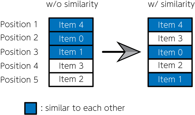
E-commerce sites with billing systems, such as product sales, hotel reservations, and music and video streaming sites, have become familiar with us today. These sites list a wide variety of items. One of the most important issue on these websites is how to decide which items to list and how to arrange them. That problem directly affects sales on e-commerce sites. If items are simply ordered by popularity (e.g., number of sales), highly similar items are often placed consecutively, which may lead to a bias toward a specific preference. Therefore, Nishimura et al. (2019) formulated the item listing problem as a quadratic assignment problem, using penalties for items with high similarity being placed next to each other. They then solved the problem with quantum annealing and succeeded in creating an item list that simultaneously accounts for item popularity and diversity. In this article, we implement the mathematical model using JijModeling, and solve it using JijZept.

A mathematical model

Let us consider which items are listed in which positions on a given website. We define the set of items to be listed as $I$ and the set of positions where items are listed as $J$. We use a binary variable $x_{i, j} = 1$ that represents to assign item $i$ to position $j$, and $x_{i, j} = 0$ otherwise.

Ensure that only one item is allocated to each position

$$\sum_{j \in J} x_{ij} = 1 \qquad (\forall i) \tag{1}$$

Ensure that only one position is allocated to each item

$$\sum_{i \in I} x_{ij} = 1 \qquad (\forall j) \tag{2}$$

An objective function

$s_{ij}$ is the estimated sales of an item $i \in I$ when it is placed in a position $j \in J$, then total estimated sales for all items is

$$\max \quad \sum_{i \in I} \sum_{j \in J} s_{ij} x_{ij} \tag{3}$$

However, as mentioned above, the objective function (3) leads a result in listing only items of the same preference, obtaining a solution that cannot be considered an optimal arrangement. Therefore, we introduce the following term in the objective function.

$$D(\mathbf{x}) = - \sum_{i \in I} \sum_{i' \in I} \sum_{j \in J} \sum_{j' \in J} f_{ii'} d_{jj'} x_{ij} x_{i'j'} \tag{4}$$

where $f_{ii'}$ is the items' similarity degree between item $i$ and $i'$, and $d_{jj'}$ is the adjacent flag of the position $j$ and $j'$; $d_{jj'} = 1$ is for the adjacent positions, otherwise $d_{jj'} =0$. By introducing this term into above objective function, we can get results in which items with small similarity are lined up in adjacent positions. From the above discussion, the function we have to maximize in this optimization problem is expressed as follows:

$$\max \quad \sum_{i \in I} \sum_{j \in J} s_{ij} x_{ij}- w \sum_{i \in I} \sum_{i' \in I} \sum_{j \in J} \sum_{j' \in J} f_{ii'} d_{jj'} x_{ij} x_{i'j'} \tag{5}$$

where $w$ represents a weight of second term.

Decomposition Methods for Item Listing Problem

In the case of a large problem, it is unlikely that feasible solutions are obtained. Therefore, we first solve the optimization problem with equation (3) as the objective function. Then, we solve the problem using equation (5) for the upper positions of the item list. This scheme effectively determines the items that are browsed most often.

Let's coding!

Let's implement a script for solveing this problem using JijModeling and JijZept.

Defining variables

We define the variables to be used for optimization. First, we consider the implementation of the mathematical model using equation (3) as the objective function.

import jijmodeling as jm

# define variables
I = jm.Placeholder('I')
J = jm.Placeholder('J')
s = jm.Placeholder('s', ndim=2)
x = jm.BinaryVar('x', shape=(I, J))
i = jm.Element('i', belong_to=I)
j = jm.Element('j', belong_to=J)

where I, J, and s are the set of items, the set of positions, and the matrix representing the estimated sales, respectively. x is the binary variables, and i, j are the indices, respectively.

Implementation for E-commerce optimization

Then, we implement the mathematical model represented by the constraints in equation (1) and (2), and the objective function in equation (3).

# make problem
problem = jm.Problem('E-commerce', sense=jm.ProblemSense.MAXIMIZE)
# set constraint 1: onehot constraint for items
problem += jm.Constraint('onehot-items', jm.sum(j, x[i, j])==1, forall=i)
# set constraint 2: onehot constraint for position
problem += jm.Constraint('onehot-positions', jm.sum(i, x[i, j])==1, forall=j)
# set objective function 1: maximize the sales
problem += jm.sum([i, j], s[i, j]*x[i, j])

We can implement objective functions as a problem to maximize them by inputting ProblemSense.MAXIMIZE in the sense argument. We make two constraints with Constraint and use the += operator to add constraints and objective functions.
With Jupyter Notebook, we can check the mathematical model implementaed.

problem

$$\begin{array}{cccc}\text{Problem:} & \text{E-commerce} & & \\& & \max \quad \displaystyle \sum_{i = 0}^{I - 1} \sum_{j = 0}^{J - 1} s_{i, j} \cdot x_{i, j} & \\\text{{s.t.}} & & & \\ & \text{onehot-items} & \displaystyle \sum_{j = 0}^{J - 1} x_{i, j} = 1 & \forall i \in \left\{0,\ldots,I - 1\right\} \\ & \text{onehot-positions} & \displaystyle \sum_{i = 0}^{I - 1} x_{i, j} = 1 & \forall j \in \left\{0,\ldots,J - 1\right\} \\\text{{where}} & & & \\& x & 2\text{-dim binary variable}\\\end{array}$$

Creating an instance

Next, we create an instance. Here we set that the number of items is 10, and the number of positions where the items are listed is also 10. In addition, the estimated sales matrix s and similarity degree matrix f are assumed to be random.

import numpy as np

# set the number of items
inst_I = 10
inst_J = 10
inst_s = np.random.rand(inst_I, inst_J)
# set instance for similarity term
inst_f = np.random.rand(inst_I, inst_I)
triu = np.tri(inst_J, k=1) - np.tri(inst_J, k=0)
inst_d = triu + triu.T
instance_data = {'I': inst_I, 'J': inst_J, 's': inst_s, 'f': inst_f, 'd': inst_d}

Solving with JijZept

We solve this problem using simulated annealing approach with JijZept.

import jijzept as jz

# set sampler
sampler = jz.JijSASampler(config='../config.toml')
# set multipliers
multipliers = {'onehot-items': 1.0, 'onehot-positions': 1.0}
# solve problem
results = sampler.sample_model(problem, instance_data, search=True, num_reads=100)

The mathematical model has two constraints, so we set the hyperparameters for thier weights as a dictionary type.

Extracting a fasible solution

We pick out the feasible and minimum energy solution from the computation results.

# get feasible solutions
feasibles = results.feasible()    
if feasibles.evaluation.objective != []:
    # get values of objective function
    objs = feasibles.evaluation.objective
    # get the index of minimum objective value
    min_obj_index = np.argmin(objs)
    print('obj: {}'.format(objs[min_obj_index]))
    # get binary array from minimum objective solution
    item_indices, position_indices = feasibles.record.solution['x'][min_obj_index][0]
    # initialize binary array
    pre_binaries = np.zeros([inst_I, inst_J], dtype=int)
    # input solution into array
    pre_binaries[item_indices, position_indices] = 1
    # format solution for visualization
    pre_zip_sort = sorted(zip(np.where(np.array(pre_binaries))[1], np.where(np.array(pre_binaries))[0]))
    for pos, item in pre_zip_sort:
        print('{}: item {}'.format(pos, item))
    # compute similarity for comparison later
    A = np.dot(instance_data['f'], pre_binaries)
    B = np.dot(pre_binaries, instance_data['d'])
    AB = A * B
    pre_similarity = np.sum(AB)
else:
    print('No feasibles solution')    

obj: -8.565938622726181
0: item 0
1: item 7
2: item 6
3: item 8
4: item 2
5: item 9
6: item 1
7: item 3
8: item 5
9: item 4

Decomposition: Leveraging penalty term and fixed variables

Earlier, we solved the problem for all varialbes. Next, we further solve the problem with the objective function in equation (5), which takes into account item similarity for the top positions. To this purpose, we define new variables.

# set variables for sub-problem
fixed_IJ = jm.Placeholder('fixed_IJ', ndim=2)
f = jm.Placeholder('f', ndim=2)
d = jm.Placeholder('d', ndim=2)
k = jm.Element('k', belong_to=I)
l = jm.Element('l', belong_to=J)
fixed_ij = jm.Element('fixed_ij', belong_to=fixed_IJ)

fixed_IJ represents the set of indices that fix the variables, which means they are not solved in the next execution. This is expressed as a two-dimensional list e.g. fixed_IJ = [[5, 6], [7, 8]] represents $x_{5, 6} = 1, x_{7, 8} = 1$. f is the item similarity matrix, d is the adjacent flag matrix. k, l and fixed_ij are new indices. Next, we add a term to minimize the sum of the similarity.

# set penalty term 2: minimize similarity
problem += jm.CustomPenaltyTerm('similarity', jm.sum([i, j, k, l], f[i, k]*d[j, l]*x[i, j]*x[k, l]))

Here we utilize CustomPenaltyTerm to represent the penalty term for similarity. We can use this for soft constraints, where we want that to be zero as much as possible, but not necessarily zero. Finally, we fix the variables for the items that appear lower positions in the optimization results before. We only optimize for the top positions again.

# set fixed variables
problem += jm.Constraint('fix', x[fixed_ij[0], fixed_ij[1]]==1, forall=fixed_ij)

We can describe fixing variables as a trivial constraint via Constraint.
Let's display the added terms with Jupyter Notebook.

problem

$$\begin{array}{cccc}\text{Problem:} & \text{E-commerce} & & \\& & \max \quad \displaystyle \sum_{i = 0}^{I - 1} \sum_{j = 0}^{J - 1} s_{i, j} \cdot x_{i, j} & \\\text{{s.t.}} & & & \\ & \text{fix} & \displaystyle x_{fixed_ij_{0}, fixed_ij_{1}} = 1 & \forall fixed_ij \in fixed_IJ \\ & \text{onehot-items} & \displaystyle \sum_{j = 0}^{J - 1} x_{i, j} = 1 & \forall i \in \left\{0,\ldots,I - 1\right\} \\ & \text{onehot-positions} & \displaystyle \sum_{i = 0}^{I - 1} x_{i, j} = 1 & \forall j \in \left\{0,\ldots,J - 1\right\} \\\text{{penalty terms}} & & & \\ & \text{similarity} & \displaystyle \sum_{i = 0}^{I - 1} \sum_{j = 0}^{J - 1} \sum_{k = 0}^{I - 1} \sum_{l = 0}^{J - 1} f_{i, k} \cdot d_{j, l} \cdot x_{i, j} \cdot x_{k, l} & \\\text{{where}} & & & \\& x & 2\text{-dim binary variable}\\\end{array}$$

Next, we create instances for fixed variables.

# set instance for fixed variables
reopt_N = 5
fixed_indices = np.where(np.array(position_indices)>=reopt_N)
fixed_items = np.array(item_indices)[fixed_indices]
fixed_positions = np.array(position_indices)[fixed_indices]
instance_data['fixed_IJ'] = [[x, y] for x, y in zip(fixed_items, fixed_positions)]

Then we set the multipliers for new penalty and constraint and perform the optimization computation with JijZept.

# set multipliers for fixed variables
multipliers['similarity'] = 1.0
multipliers['fixed'] = 1.0
# solve sub-problem
results = sampler.sample_model(problem, instance_data, search=True, num_reads=100)

Again, we extract a feasible solution from the results and display it.

# get feasible solutions
feasibles = results.feasible()
if feasibles.evaluation.objective != []:
    # get values of objective function
    objs = feasibles.evaluation.objective
    # get values of penalty term
    penals = feasibles.evaluation.penalty['similarity']
    # find the index of minimum objective + penalty
    sums = objs + penals
    min_sum_index = np.argmin(sums)
    print('obj: {}, penalty: {}'.format(objs[min_sum_index], penals[min_sum_index]))
    # get binary array from minimum objective solution
    item_indices, position_indices = feasibles.record.solution['x'][min_sum_index][0]
    # initialize binary array
    post_binaries = np.zeros([inst_I, inst_J], dtype=int)
    # input solution into array
    post_binaries[item_indices, position_indices] = 1
    # format solution for visualization
    post_zip_sort= sorted(zip(np.where(np.array(post_binaries))[1], np.where(np.array(post_binaries))[0]))
    for i, j in post_zip_sort:
        print('{}: item {}'.format(i, j))
    # get similarity 
    post_similarity = feasibles.evaluation.penalty["similarity"][min_sum_index]
else:
    print('No feasibles solution')

obj: -8.136738402512211, penalty: 8.217841645587898
0: item 0
1: item 7
2: item 8
3: item 6
4: item 2
5: item 9
6: item 1
7: item 3
8: item 5
9: item 4

Let us compare these two results.

items = ["Item {}".format(i) for i in np.where(pre_binaries==1)[0]]
pre_order = np.where(pre_binaries==1)[1]
post_order = np.where(post_binaries==1)[1]

To plot a graph, we define the following class.

from typing import Optional
import matplotlib.pyplot as plt

class Slope:
    """Class for a slope chart"""
    def __init__(self,
        figsize: tuple[float, float] = (6,4),
        dpi: int = 150,
        layout: str = 'tight',
        show: bool =True,
        **kwagrs):

        self.fig = plt.figure(figsize=figsize, dpi=dpi, layout=layout, **kwagrs)
        self.show = show

        self._xstart: float = 0.2
        self._xend: float = 0.8
        self._suffix: str = ''
        self._highlight: dict = {}
        
    def __enter__(self):
        return(self)

    def __exit__(self, exc_type, exc_value, exc_traceback):
        plt.show() if self.show else None
        
    def highlight(self, add_highlight: dict) -> None:
        """Set highlight dict
        
        e.g.
            {'Group A': 'orange', 'Group B': 'blue'}
        
        """
        self._highlight.update(add_highlight)
        
    def config(self, xstart: float =0, xend: float =0, suffix: str ='') -> None:
        """Config some parameters
        
            Args:
                xstart (float): x start point, which can take 0.0〜1.0        
                xend (float): x end point, which can take 0.0〜1.0
                suffix (str): Suffix for the numbers of chart e.g. '%'
        
            Return:
                None
                
        """
        self._xstart = xstart if xstart else self._xstart
        self._xend = xend if xend else self._xend
        self._suffix = suffix if suffix else self._suffix
    
    def plot(self, time0: list[float], time1: list[float], 
             names: list[float], xticks: Optional[tuple[str,str]] = None, 
             title: str ='', subtitle: str ='', ):
        """Plot a slope chart
        
        Args:
            time0 (list[float]): Values of start period
            time1 (list[float]): Values of end period
            names (list[str]): Names of each items
            xticks (tuple[str, str]): xticks, default to 'Before' and 'After'
            title (str): Title of the chart
            subtitle (str): Subtitle of the chart, it might be x labels
        
        Return:
            None
        
        """
        
        xticks = xticks if xticks else ('Before', 'After')
        
        xmin, xmax = 0, 4
        xstart = xmax * self._xstart
        xend = xmax * self._xend
        ymax = max(*time0, *time1)
        ymin = min(*time0, *time1)
        ytop = ymax * 1.2
        ybottom = ymin - (ymax * 0.2)
        yticks_position = ymin - (ymax * 0.1)
        
        text_args = {'verticalalignment':'center', 'fontdict':{'size':10}}
        
        for t0, t1, name in zip(time0, time1, names):
            color = self._highlight.get(name, 'gray') if self._highlight else None
            
            left_text = f'{name} {str(round(t0))}{self._suffix}'
            right_text = f'{str(round(t1))}{self._suffix}'
            
            plt.plot([xstart, xend], [t0, t1], lw=2, color=color, marker='o', markersize=5)
            plt.text(xstart-0.1, t0, left_text, horizontalalignment='right', **text_args)
            plt.text(xend+0.1, t1, right_text, horizontalalignment='left', **text_args)
        
        plt.xlim(xmin, xmax)
        plt.ylim(ytop, ybottom)
    
        plt.text(0, ytop, title, horizontalalignment='left', fontdict={'size':15})
        plt.text(0, ytop*0.95, subtitle, horizontalalignment='left', fontdict={'size':10})
        
        plt.text(xstart, yticks_position, xticks[0], horizontalalignment='center', **text_args)
        plt.text(xend, yticks_position, xticks[1], horizontalalignment='center', **text_args)
        plt.axis('off')
        
        
def slope(
    figsize=(6,4),
    dpi: int = 150,
    layout: str = 'tight',
    show: bool =True,
    **kwargs
    ):
    """Context manager for a slope chart"""
    
    slp = Slope(figsize=figsize, dpi=dpi, layout=layout, show=show, **kwargs)

    return slp

Then, we display a graph for comparison.

pre_string = "Similarity: {:.2g}".format(pre_similarity)
post_string = "Similarity: {:.2g}".format(post_similarity)
with slope() as slp:
    slp.plot(pre_order, post_order, items, (pre_string, post_string))

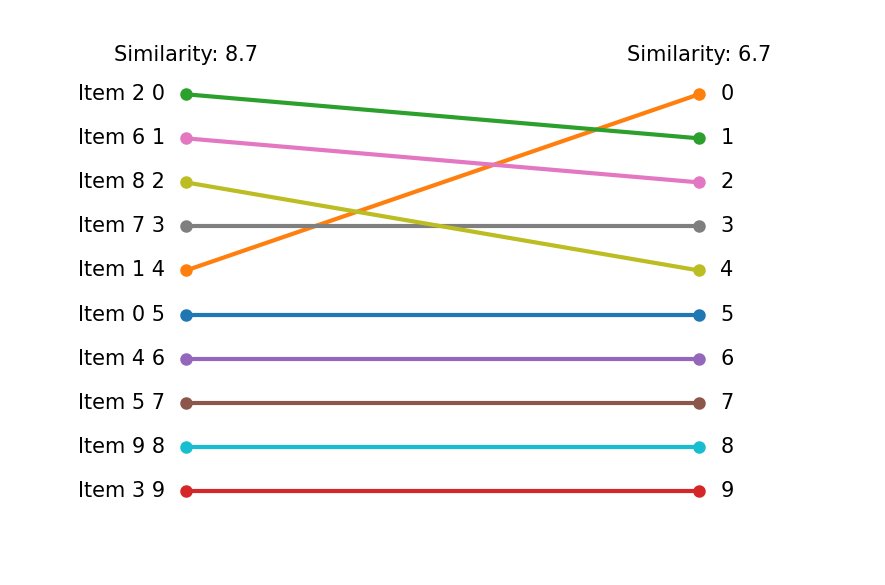
The left and right columns show the results without and with similarity term, respectively. The lower positions remain unchanged due to fixing variables. However, we can see the change in upper positions due to the similarity.

References

• Nishimura et al., 2019, "Item Listing Optimization for E-Commerce Websites Based on Diversity"