The K-Median Problem

The k-median problem is the problem of clustering data points into k clusters, aiming to minimize the sum of distances between points belonging to a particular cluster and the data point that is the center of the cluster. This can be considered a variant of k-means clustering. For k-means clustering, we determine the mean value of each cluster whereas for k-median we use the median value. This problem is known as NP-hard. We describe how to implement the mathematical model of k-median problem with JijModeling and solve it with JijZept.

Mathematical Model

Let us consider a mathematical model for k-median problem.

Decisioin variables

We denote $x_{i, j}$ to be a binary variable which is 1 if $i$-th data point belongs to the $j$-th median data point and 0 otherwise. We also use a binary variable $y_j$ which is 1 if $j$-th data point is the median and 0 otherwise.

$$x_{i,j} = \begin{cases} 1,~\text{Node $i$ is covered by median $j$}\\ 0,~\text{Otherwise} \end{cases}$$

$$y_j = \begin{cases} 1,~\text{Node $j$ is a median.}\\ 0,~\text{Otherwise} \end{cases}$$

Mathematical Model

Our goal is to find a solution that minimizes the sum of the distance between $i$-th data point and $j$-th median point. We also set three constraints:

1. A data point must belong to some single median data point,
2. the number of median points is $k$,
3. the data points must belong to a median point.

These can be expressed in a mathematical model as follows.

$$\begin{aligned} \min_x &\sum_{i}\sum_j d_{i,j}x_{i,j} \\ \mathrm{s.t.}~&\sum_{j} x_{i,j} = 1,~\forall i\\ &\sum_j y_j = k\\ &x_{i,j} \leq y_j, ~\forall i, j\\ &x_{i,j} \in \{0, 1\} ~\forall i, j\\ &y_j \in \{0, 1\}~\forall j \end{aligned} \tag{1}$$

Modeling by JijModeling

Here, we show an implementation using JijModeling. We first define variables for the mathematical model described above.

import jijmodeling as jm

d = jm.Placeholder("d", ndim=2)
N = d.len_at(0, latex="N")
J = jm.Placeholder("J", ndim=1)
k = jm.Placeholder("k")
i = jm.Element("i", belong_to=(0, N))
j = jm.Element("j", belong_to=J)
x = jm.BinaryVar("x", shape=(N, J.shape[0]))
y = jm.BinaryVar("y", shape=(J.shape[0],))

d is a two-dimensional array representing the distance between each data point and the median point. The number of data points N is extracted from the number of elements in d. J is a one-dimensional array representing the candidate indices of the median point. k is the number of median points. i and j denote the indices used in the binary variables, respectively. Finally, we define the binary variables x and y.

Then, we implement (1).

problem = jm.Problem("k-median")
problem += jm.sum([i, j], d[i, j]*x[i, j])
problem += jm.Constraint("onehot", x[i, :].sum() == 1, forall=i)
problem += jm.Constraint("k-median", y[:].sum() == k)
problem += jm.Constraint("cover", x[i, j] <= y[j], forall=[i, j])

With jm.Constraint("onehot", x[i, :].sum() == 1, forall=i), we insert as a constraint that $\sum_j x_{i, j} = 1$ for all $i$. jm.Constraint("k-median", y[:].sum() == k) represents $\sum_j y_j = k$. jm.Constraint("cover", x[i, j] <= y[j], forall=[i, j]) requires that $x_{i, j} \leq y_j$ must be for all $i, j$.

We can check the implementation of the mathematical model on Jupyter Notebook.

problem

$\begin{array}{cccc}\text{Problem:} & \text{k-median} & & \\& & \min \quad \displaystyle \sum_{i = 0}^{N - 1} \sum_{j \in J} d_{i, j} \cdot x_{i, j} & \\\text{{s.t.}} & & & \\ & \text{cover} & \displaystyle x_{i, j} \leq y_{j} & \forall i \in \left\{0,\ldots,N - 1\right\} \forall j \in J \\ & \text{k-median} & \displaystyle \sum_{\ast_{0} = 0}^{\mathrm{len}\left(J, 0\right) - 1} y_{\ast_{0}} = k & \\ & \text{onehot} & \displaystyle \sum_{\ast_{1} = 0}^{\mathrm{len}\left(J, 0\right) - 1} x_{i, \ast_{1}} = 1 & \forall i \in \left\{0,\ldots,N - 1\right\} \\\text{{where}} & & & \\& y & 1\text{-dim binary variable}\\& x & 2\text{-dim binary variable}\\\end{array}$

Prepare instance

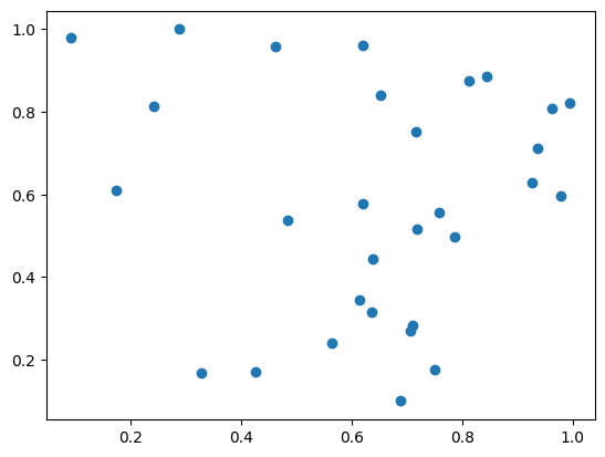
We prepare and visualize data points.

import matplotlib.pyplot as plt
import numpy as np

num_nodes = 30
X, Y = np.random.uniform(0, 1, (2, num_nodes))

plt.plot(X, Y, "o")

[<matplotlib.lines.Line2D at 0x7f1a6b7463d0>]

We need to calculate the distance between each data point.

XX, XX_T = np.meshgrid(X, X)
YY, YY_T = np.meshgrid(Y, Y)
distance = np.sqrt((XX - XX_T)**2 + (YY - YY_T)**2)

ph_value = {
    "d": distance,
    "J": np.arange(0, num_nodes),
    "k": 4
}

Solve with JijZept

We solve the problems implemented so far using JijZept JijSASampler. We also use the parameter search function by setting search=True here.

import jijzept as jz

sampler = jz.JijSASampler(config="config.toml")
response = sampler.sample_model(problem, ph_value, multipliers={"onehot": 1.0, "k-median": 1.0, "cover": 1.0}, search=True)

From the results, we extract the feasible solutions and show the smallest value of the objective function among them.

# get sampleset
sampleset = response.get_sampleset()
# extract feasible solutions
feasible_samples = sampleset.feasibles()
# get the value of feasible objective function
feasible_objectives = [sample.eval.objective for sample in feasible_samples]
# get the lowest value of objective function
lowest_index = np.argmin(feasible_objectives)
# show the result
print(lowest_index, feasible_objectives[lowest_index])

0 6.622000297366702

From the binary variable $y_j$, which data point is used as the median, we get the indices of the data points that are actually used as the median.

# check the solution
y_indices = feasible_samples[lowest_index].var_values["y"].values.keys()
median_indices = np.array([index[0] for index in y_indices])
print(median_indices)

[25  1 19 20]

This information allows us to visualize how data points are clustered.

median_X, median_Y = X[median_indices], Y[median_indices]

d_from_m = []
for m in median_indices:
    d_from_m.append(np.sqrt((X - X[m])**2 + (Y - Y[m])**2))

cover_median = median_indices[np.argmin(d_from_m, axis=0)]

plt.plot(X, Y, "o")
plt.plot(X[median_indices], Y[median_indices], "o", markersize=10)
for index in range(len(X)):
    j_value = cover_median[index]
    i_value = index
    plt.plot(X[[i_value, j_value]], Y[[i_value, j_value]], c="gray")

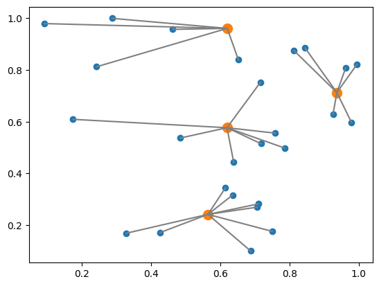
Orange and blue points show the median and other data points respectively. The gray line connects the median and the data points belonging to that cluster. This figure shows how they are into clusters.