Graph Partitioning

Here we show how to solve the graph partitioning problem using JijZept and JijModeling. This problem is also mentioned in 2.2. Graph Partitioning on Lucas, 2014, "Ising formulations of many NP problems".

What is Graph Partitioning?

Graph partitioning is the problem of dividing a graph into two subsets of equal size with the aim of minimizing the number of edges between the subsets.

Example

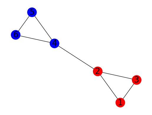
Let us take a look at the following situation. Consider a graph with 6 vertices labeled from 1 to 6, and edges connecting vertices as follows:

• 1 is connected to 2 and 3
• 2 is connected to 1, 3, and 4
• 3 is connected to 1 and 2
• 4 is connected to 2, 5, and 6
• 5 is connected to 4 and 6
• 6 is connected to 4 and 5

The goal is to partition this graph into two subsets of equal size (i.e., 3 vertices in each subset) with minimized edges between them. In this case, the optimal solution is $\{1, 2, 3\}, \{4, 5, 6\}$, where there is only 1 edge connecting vertices in different subsets (i.e., the edge (2,4)), which is the minimum possible number of edges connecting the two subsets.

Mathematical Model

Let $G=(V, E)$ be the undirected graph where $V$ is the set of vertices and $E$ is the set of edges. The goal is to partition $V$ into two subsets $V_1$ and $V_2$ of equal size, with the number of edges crossing the partition being minimized. We introduce variables $x_{u}$ which is 1 if vertex $u$ is in the subset $V_1$ and 0 if vertex $u$ is in the subset $V_2$.

Constraint: the vertices must be partitioined into two equal-sized sets

We express this constraint as follows:

$$∑_{u \in V} x_u = V/2 \tag{1}$$

Objective function: minimize the number of edges crossing the partition

$$\min \quad \sum_{(uv) \in E} (\{x_{u} (1-x_{v})\}+\{(1-x_{u}) x_{v}\}) \tag{2}$$

Here, the first term $x_u (1 - x_v)$ evaluates to 1 if edge (u, v) crosses the boundary between $V_1$ and $V_2$ (i.e., if $u$ belongs to $V_2$ and $v$ belongs to $V_1$), and 0 otherwise. Similarly, the second term $(1 - x_u) x_v$ evaluates to 1 if edge (u, v) crosses the boundary between $V_1$ and $V_2$ (i.e., if $u$ belongs to $V_1$ and $v$ belongs to $V_2$), and 0 otherwise.

Thus, this objective function is an indicator of how much graph partitioning has been achieved.

Modeling by JijModeling

Next, we show an implementation using JijModeling. We first define variables for the mathematical model described above.

import jijmodeling as jm

# define variables
V = jm.Placeholder('V')
E = jm.Placeholder('E', ndim=2)
x = jm.BinaryVar('x', shape=(V,))
u = jm.Element('u', belong_to=V)
e = jm.Element('e', belong_to=E)

V=jm.Placeholder('V') represents the number of vertices. We denote E=jm.Placeholder('E', ndim=2) as a set of edges. Then, we define a list of binary variables x=jm.BinaryVar('x', shape=(V,)), and we set the subscripts u used in the mathematical model. Finally, e represents the variable for edges. e[0] and e[1] represent the two vertices connected by the edge.

Constraint

We implement a constraint Equation (1).

# set problem
problem = jm.Problem('Graph Partitioning')
# set constraint: the vertices must be partitioined into two equal-sized sets
const = jm.sum(u, x[u])
problem += jm.Constraint('constraint', const==V/2)

Objective function

Next, we implement an objective function Equation (2).

# set objective function: minimize the number of edges crossing the partition
A_1 = x[e[0]]*(1-x[e[1]])
A_2 = (1-x[e[0]])*x[e[1]]
problem += jm.sum(e, (A_1 + A_2))

Let's display the implemented mathematical model in Jupyter Notebook.

problem

$\begin{array}{cccc}\text{Problem:} & \text{Graph Partitioning} & & \\& & \min \quad \displaystyle \sum_{e \in E} \left(x_{e_{0}} \cdot \left(- x_{e_{1}} + 1\right) + \left(- x_{e_{0}} + 1\right) \cdot x_{e_{1}}\right) & \\\text{{s.t.}} & & & \\ & \text{constraint} & \displaystyle \sum_{u = 0}^{V - 1} x_{u} = V \cdot 2^{(-1)} & \\\text{{where}} & & & \\& x & 1\text{-dim binary variable}\\\end{array}$

Prepare an instance

We prepare a graph using NetworkX. Here we create random graph with 12 vertices.

import networkx as nx

# set the number of vertices
inst_V = 12
# create a random graph
inst_G = nx.gnp_random_graph(inst_V, 0.4)
# get information of edges
inst_E = [list(edge) for edge in inst_G.edges]
instance_data = {'V': inst_V, 'E': inst_E}

Solve by JijZept's SA

We solve this problem using JijZept JijSASampler. We also use the parameter search function by setting search=True.

import jijzept as jz

# set sampler
config_path = "config.toml"
sampler = jz.JijSASampler(config=config_path)
# solve problem
response = sampler.sample_model(problem, instance_data, multipliers={"constraint": 0.5}, num_reads=100, search=True)

Visualize the solution

In the end, we extract the lowest energy solution from the feasible solutions and visualize it.

import matplotlib.pyplot as plt
import numpy as np

# get sampleset which is returned from JijZept
sampleset = response.get_sampleset()
# extract feasible samples
feasible_samples = sampleset.feasibles()
# get the values of feasible objective function
feasible_objectives = [sample.eval.objective for sample in feasible_samples]

if len(feasible_objectives) == 0:
    print("No feasible sample found ...")
else:
    # get the lowest index
    lowest_index = np.argmin(feasible_objectives)
    print("Objective: ", feasible_objectives[lowest_index])
    # get the solution of lowest index
    lowest_solution = feasible_samples[lowest_index].var_values["x"].values
    # get the index of x == 1
    x_indices = [key[0] for key in lowest_solution.keys()]
    # set color list for visualization
    cmap = plt.get_cmap("tab10")
    # initialize vertex color list
    node_colors = [cmap(0)] * instance_data["V"]
    # set vertex color list
    for i in x_indices:
        node_colors[i] = cmap(1)
    # make figure
    nx.draw_networkx(inst_G, node_color=node_colors, with_labels=True)
    plt.show()

Objective:  5.0

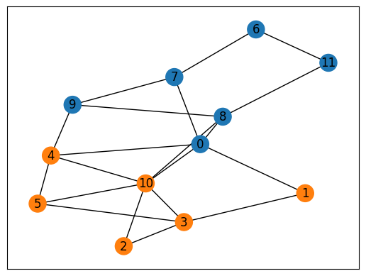
With the above visualization, we obtain a feasible partitioning for this graph.