Dynamic Asset Allocation with Expected Shortfall

Introduction

The probability of not reaching a target asset amount or investment return on an investment is called shortfall risk. Introducing a measure of expected shortfall risk in portfolio optimization makes it possible to consider returns even in extreme models where the market moves dynamically. Xu et al. (2023) treated target returns as constraints in the Markowitz portfolio optimization model and proposed an iterative algorithm that dynamically adjusts target returns to meet target shortfalls. In this article, we use JijModeling and JijZept to implement this algorithm.

Dynamic Asset Allocation

The dynamic asset allocation problem is the problem of allocating/investing funds in $N$ assets to meet expected returns while keeping risk below a given threshold. A $N \times D_\mathrm{total}$ matrix $R$ representing the returns are obtained from the finance data. $N$ is the number of stocks to be covered and $D_\mathrm{total}$ is the number of days data are collected. We divide $R$ into the period of $T$ days and index the data for each time period. For example, $R_t$ represents the return data from $t$-th period. $\mu_t$ is the mean value calculated from $R_t$. Using these quantities, the covariance matrix of $t$-th period $C_t$ is calculated as

$$C_{t, i, j} = \frac{(\mathbf{e}_i^\top R_t - \mu^\top_{t, i} \mathbf{1}) \cdot (\mathbf{e}_j^\top R_t - \mu^\top_{t, j} \mathbf{1})}{T-1} \tag{1}$$

where $\mathbf{e}_i$ is a column vector of all zeros except with a one at the $j$-th position. Asset allocation could be a challenging problem during periods of unpredictable market turbulence. Therefore, we should set a threshold to avoid risk during those periods. The risk threshold can be set using observed market metrics from a volatile time period, for example, the 2008 market crash. Major methods of risk measurement include:

• Volatility: the standard deviation of the portfolio return.
• Value-at-Risk at level $\alpha$: the smallest number $y$ such that the probability that a portfolio does not lose more than $y$ of total budget is at least $1−α$.
• Expected Shortfall at level $\alpha$: the expected return from the worst $\alpha$% cases.

In the following sections, we focus on the expected shortfall as our risk measurement and consider a formulation for portfolio optimization problem.

Expected Shortfall based Portfolio Optimization

The expected shortfall al level $\alpha$ is defined as:

$$\mathrm{ES}_\alpha (w_t, R_t) = \mathrm{mean}(\mathrm{lowest} \ \alpha \% \ \mathrm{from} \ w_t^\top R_t) \tag{2}$$

where the weight vector $w_t$ indicates what fraction of the budget is invested in each asset in the $t$th period. We minimize the expected shortfall, which is the worst-case average. Therefore, portfolio optimization considering expected shortfall becomes a problem of minimizing the expected shortfall $\mathrm{ES}_\alpha$ under the constraints that the expected return is satisfied, the variance of the portfolio is small, and all assets are invested. However, the expected shortfall cannot be expressed by a quadratic formulation natively. If we reformulate it to QUBO, it is necessary to introduce new auxiliary variables. Therefore, to avoid this difficulty, we treat the expected shortfall as the convergence criterion. To do this approach, assuming that the assets’ historical returns follow a Gaussian distribution, we can approximate the expected shortfall of a given portfolio $P$ by

$$\mathrm{ES}_\alpha (P) = \mu + \sigma \frac{\phi (\Phi^{-1} (\alpha))}{1-\alpha} \tag{3}$$

where $\mu$ is the expected return, $\sigma$ is the volatility of the portfolio, and $\phi(x)$ and $\Phi(x)$ are the Gaussian probability distribution and cumulative distribution functions, respectively.
We use this criterion as the market risk. For example, if the risk is small, we make a slightly larger investment to get a larger return. Conversely, during periods of market turbulence and high risk, we take a lower risk of losing money in exchange for a smaller return. In order to dynamically vary returns in accordance with the expected shortfall for a given period, Xu et al. (2023) proposed the following algorithm.

Algorithm: Expected Shortfall based Dynamic Asset Allocation during period $t$
Input: $\mu_t, R_t, \sigma_\mathrm{ref}, \sigma_{\mathrm{ref}, t}, \mathrm{ES}_\mathrm{ref}, \alpha$
Output: $w_t$
1: $p_t = \mathrm{mean} (\mu_t)$. // Initialize the target return
2: $\mathrm{EST}_t = \frac{\sigma_\mathrm{ref}}{\sigma_{\mathrm{ref}, t}} \mathrm{ES}_\mathrm{ref}$. // Initialize the target expected shortfall
3: $C_t = \mathrm{cov}(R_t)$ // Compute the co-variance matrix from the returns
4: while True do:
5:   if $p_t > \max (\mu_t)$:
6:     return 0. // Return constraint cannot be satisfied
7:   $w_t$ = Markowitz($\mu_t, C_t, p_t$). // Solve Markowitz formulation with annealing
8:   $\mathrm{ES}_t = \mathrm{ES}_\alpha (w_t, R_t)$. // Compute the expected shortfall using eq.(2)
9:   if $\frac{\mathrm{ES}_t}{\mathrm{EST}_t} > 1 + \epsilon$:
10:    $p_t = p_t (1-\delta)$. // Decrease target return for lower risks
11:  else if: $\frac{\mathrm{ES}_t}{\mathrm{EST}_t} < 1-\epsilon$
12:    $p_t = p_t (1+\delta)$. // Increase target return as there is room for more risks
13:  else:
14:    return $w_t$

where $\sigma_\mathrm{ref}$ is the volatility of a reference asset's returns during the market crash in 2008. $\sigma_{\mathrm{ref}, t}$ is the volatility of the reference asset's returns during the $t$-th period. $\mathrm{ES}_\mathrm{ref}$ is the reference asset's expected shortfall during the market crash. $\mathrm{EST}_t$ is the target expected shortfall at the $t$-th period. $\alpha$ is the risk level parameter. $\mathrm{ES}_t$ is the expected shortfall for the computed portfolio during the optimization process at $t$-th period. $\epsilon$ is the error tolerance parameter, and $\delta$ is the momentum parameter that is adjusted dynamically. The Markowitz optimization problem can be expressed by the quadratic optimization problem as:

$$\begin{align} \min_w & \quad w_t^\top C_t w_t \\ \mathrm{s.t.} & \quad \mu_t^\top w_t \geq p_t \\ & \quad \sum_i w_{t, i} = 1, \quad w_{t, i} \geq 0 \quad (\forall i) \end{align} \tag{4}$$

For simplicity, we set $w_{t, i}$ are binary variables in $\{0, 1\}$. From the constraint $\sum_i w_{t, i} = 1$, we concentrate our assets in one stock, and aim the return is always greater than $p_t$.

Let's coding!

Here, we implement a script that solves this problem using JijModeling and JijZept.

Defining variables

We define the variables for eq.(4).

import jijmodeling as jm

# define variables
N = jm.Placeholder('N')
p = jm.Placeholder('p')
mu = jm.Placeholder('mu', ndim=1)
C = jm.Placeholder('C', ndim=2)
w = jm.BinaryVar('w', shape=(N, ))
i = jm.Element('i', belong_to=N)
j = jm.Element('j', belong_to=N)

N is the total number of stocks, p is the lower liimit of return $p_t$, mu is the return $\mu_t$ for each stock, and C is the covariance matrix $C_t$. w is the binary variable for optimization, and i and j are the indices, respectively.

Implementing Markowitz formulation

Next, we implement Markowitz mathematical model eq.(3).

# set a problem
problem = jm.Problem('shortfall')
# constraint 1: ensure the target return
problem += jm.Constraint('return', jm.sum(i, mu[i]*w[i])>=p)
# constraint 2: buy a stock
problem += jm.Constraint('onehot', jm.sum(i, w[i])==1)
# objective function: minimize variance
problem += jm.sum([i, j], C[i, j]*w[i]*w[j])

We generate a problem with Problem and then implement two constraints with Constraint. We can implement the sum in two subscripts at once by using sum([i, j], ...).
With Jupyter Notebook, we can check the mathematical model implemented.

problem

$$\begin{array}{cccc}\text{Problem:} & \text{shortfall} & & \\& & \min \quad \displaystyle \sum_{i = 0}^{N - 1} \sum_{j = 0}^{N - 1} C_{i, j} \cdot w_{i} \cdot w_{j} & \\\text{{s.t.}} & & & \\ & \text{onehot} & \displaystyle \sum_{i = 0}^{N - 1} w_{i} = 1 & \\ & \text{return} & \displaystyle \sum_{i = 0}^{N - 1} mu_{i} \cdot w_{i} \geq p & \\\text{{where}} & & & \\& w & 1\text{-dim binary variable}\\\end{array}$$

Solving with JijZept

We solve Markowitz portfolio optimization using simulated annealing approach with JijZept.

import jijzept as jz

# set sampler
sampler = jz.JijSASampler(config='../config.toml')
# set multipliers
multipliers = {'return': 1.0, 'onehot': 1.0}

In this problem, we have two constraints. Therefore, we specify each multiplier in dictionary type.
Next, we implement subroutines to execute the algorithm proposed by Xu et al. (2023).

import numpy as np
from scipy.stats import norm

# a function to compute reference vlatility and expected shortfall
def compute_reference(ref_asset, ref_start_date, ref_end_date, alpha):
    ref_data = web.DataReader(ref_asset, ref_start_date, ref_end_date)['Close']
    ref_volatility = ref_data.std()
    ref_mean = ref_data.mean()
    ref_expected_shortfall = ref_mean + ref_volatility * norm.pdf(norm.ppf(alpha)) / (1-alpha)
    return ref_volatility, ref_expected_shortfall

# a function to extract a solution from results
def extract_solution(results, N):
    # get feasible solutions
    feasibles = results.feasible()
    if feasibles.evaluation.objective == []:
        print('No feasibles solution')
    else:
        # get values of objective function
        objs = feasibles.evaluation.objective
        # get the index of minimum objective value
        min_obj_index = np.argmin(objs)
        # get solution
        w = feasibles.record.solution['w'][min_obj_index]
        # convert solution to binary vector
        list_index = w[0][0]
        list_binary = np.zeros(N, dtype=int)
        list_binary[list_index] = 1
        return list_binary

# solve Markowitz optimization problem
def solve_markowitz(instance_data):
    # compute SA with JijZept
    results = sampler.sample_model(problem, instance_data, multipliers, search=True, num_reads=100)
    w_t = extract_solution(results, instance_data['N'])
    return w_t

# compute expected shortfall from result of Markowitz optimization
def compute_shortfall(alpha, w, ret, vol):
    es = np.dot(w, ret) + np.dot(w, vol) * norm.pdf(norm.ppf(alpha)) / (1-alpha)
    return es

compute_reference is a function that computes the volatility $\sigma_\mathrm{ref}$ and expected shortfall $\mathrm{ES}_\mathrm{ref}$ of the reference data, solve_markowitz is for solving the otimization problem eq.(3). extract_solution is a function that extracts the feasible and smallest objective solution from the result of solve_markowitz, and converts that solution to a binary vector. Lastly, compute_shortfall computes the expected shortfall using the portfolio obtained from solve_markowitz. Utilizing these subroutines, we implement the algorithm from Xu et al. (2023).

import datetime
import yfinance as yf
import pandas as pd
import pandas_datareader.data as web
yf.pdr_override()

# set input parameters, alpha, delta and eps
alpha = 0.99
delta = 0.1
eps = 0.25
# set start and end date for reference data
ref_start_date = datetime.date(year=2008, month=1, day=1)
ref_end_date = datetime.date(year=2009, month=1, day=1)
# compute volatility and expected shortfall from reference data
ref_volatility, ref_expected_shortfall = compute_reference('SPY', ref_start_date, ref_end_date, alpha)
# set the name of assets
list_assets = ['SPY', 'EEM', 'QQQ', 'SLV', 'SQQQ', 'XLF', 
                'AUDUSD=X', 'EURUSD=X', 'GBPUSD=X', 'CNYUSD=X', 'INRUSD=X', 'JPYUSD=X']
ref_asset_t = list_assets[0]
# set start date for data and date interval
start_date_t = datetime.date(year=2022, month=1, day=1)
dt = 14
# set the number of iteration
iteration = 6
# initialize lists for final results
list_results = []
list_shortfall = []
list_return = []
list_target = []
# main loop
for _ in range(iteration):
    # set end date
    end_date_t = start_date_t + datetime.timedelta(days=dt)
    # get reference stock data
    ref_data_for_volatility_t = web.DataReader(ref_asset_t, start_date_t, end_date_t)['Close']
    # compute volatility
    ref_volatility_t = ref_data_for_volatility_t.std()
    # compute target expected shortfall
    target_expected_shortfall_t = ref_volatility / ref_volatility_t * ref_expected_shortfall
    # initialize dataframe
    data_assets = pd.DataFrame()
    for asset in list_assets:
        # get stock data and concat 
        data = web.DataReader(asset, start_date_t, end_date_t).rename(columns={'Close': asset})
        data_assets = pd.concat([data_assets, data[asset]], axis=1)
    # if nan exists, drop
    data_assets_dropna = data_assets.dropna(how='any')
    # compute mean
    mean_t = data_assets_dropna.mean(axis=0).values
    # compute covariant matrix
    cov_t = data_assets_dropna.cov().values
    # compute volatility
    volatility_t = data_assets.std().values
    # get the number of assets
    N = len(list_assets)
    # normalize mean, covariant matrix, and pt
    mean_t_normalize = mean_t / mean_t.max()
    cov_t_normalize = cov_t / cov_t.max()
    p_t_normalize = mean_t_normalize.mean()
    instance_data = {'N': N, 'p': p_t_normalize, 'mu': mean_t_normalize, 'C': cov_t_normalize}
    while True:
        w_t = solve_markowitz(instance_data)
        if p_t_normalize > max(mean_t_normalize):
            print('Caution!!! Return constraint cannot be satisfied!!!')
            break
        expected_shortfall_from_markowitz = compute_shortfall(alpha, w_t, mean_t, volatility_t)
        if abs(expected_shortfall_from_markowitz) / abs(target_expected_shortfall_t) > 1 + eps:
            instance_data['p'] *= 1 - delta
        # elif abs(expected_shortfall_from_markowitz) / abs(target_expected_shortfall_t) < 1 - eps:
        #     instance_data['p'] *= 1 + delta
        else:
            break
    start_date_t = end_date_t
    list_results.append(w_t)
    list_shortfall.append(expected_shortfall_from_markowitz)
    list_target.append(target_expected_shortfall_t)
    list_return.append(mean_t)

Visualizing result

We plot the obtained result.

import matplotlib.pyplot as plt

list_final_ret = [np.dot(x, y) for x, y in zip(list_results, list_return)]
fig = plt.figure()
ax1 = fig.add_subplot(111)
ax1.set_xlabel('Period')
ax1.set_ylabel('Return')
ln1 = ax1.plot(list_final_ret, color='green', label='Return')
ax2 = ax1.twinx()
ax2.set_ylabel('Shortfall')
ln2 = ax2.plot(list_shortfall, color='indigo', label='Expected shortfall')
ln3 = ax2.plot(list_target, color='dodgerblue', label='Target shortfall')
h1, l1 = ax1.get_legend_handles_labels()
h2, l2 = ax2.get_legend_handles_labels()
ax1.legend(h1+h2, l1+l2, loc='lower left')

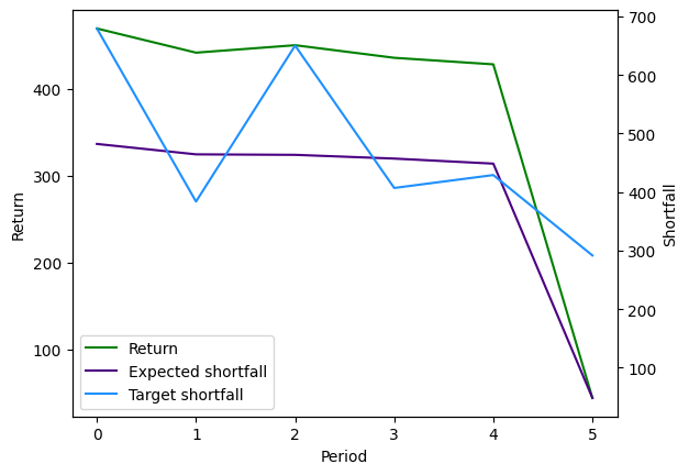
In the last period 5, the target shortfall is decreasing. The portfolio is chosen so that the expected shortfall decrease accordingly, resulting in a smaller return.

References

• Xu et al., 2023, "Dynamical Asset Allocation with Expected Shortfall via Quantum Annealing"
• Markowitz, 1952, "Portfolio Selection"