Graph Isomorphisms problem

Here we show how to solve graph isomorphisms problem using JijZept and JijModeling. This problem is also mentioned in 9. Graph Isomorphisms on Lucas, 2014, "Ising formulations of many NP problems".

What is Graph Isomorphisms Problem?

Graph isomorphism is a concept that describes when two graphs $G_1$ and $G_2$ have the same structure, meaning that they have the same $N$ number of vertices and edges and that their vertices and edges are arranged in the same way. More carefully: identical graphs are any graph $G = (V, E)$ with vertices labeled as $1,\cdots,N$ and with an $N \times N$ adjacency matrix $A$ with

$$A_{ij} \equiv \begin{cases} 1 & \text{if } (ij) \in E \\ 0 & \text{if } (ij) \notin E \end{cases}$$

which contains all information about the edge set $E$.

Mathematical Model

First, we introduce binary variables $x_{v, i}$ which are 1 if vertex $v$ in $G_2$ gets mapped to vertex $i$ in $G_1$ and 0 otherwise.

Constraint 1: the map is bijective

A bijective map between two graphs is a one-to-one correspondence between the vertices of the two graphs, such that each vertex in one graph is paired with a unique vertex in the other graph.

$$\quad \sum_{i}x_{v,i} = 1 \quad (\forall v) \tag{1}$$

$$\quad \sum_{v}x_{v,i} = 1 \quad (\forall i) \tag{2}$$

Constraint 2: no bad mapping exists

An edge that is not in $G_1$ but is in $G_2$, or an edge that is in $G_1$ but is not in $G_2$ should not exist.

$$\quad \sum_{ij \notin E_1}\sum_{uv \in E_2} x_{u,i}x_{v,j}+\sum_{ij \in E_1}\sum_{uv \notin E_2} x_{u,i}x_{v,j} = 0\tag{3}$$

Modeling by JijModeling

Next, we show an implementation using JijModeling. We first define variables for the mathematical model described above.

import jijmodeling as jm

#define variables
V = jm.Placeholder('V')  # number of vertices
E1 = jm.Placeholder('E1', ndim=2)  # set of edges
E2 = jm.Placeholder('E2', ndim=2)  # set of edges
E1_bar = jm.Placeholder('E1_bar', ndim=2)
E2_bar = jm.Placeholder('E2_bar', ndim=2)

x = jm.BinaryVar('x',shape=(V,V))
i = jm.Element('i', belong_to=(0, V))
j = jm.Element('j', belong_to=(0, V))
u = jm.Element('u', belong_to=(0, V))
v = jm.Element('v', belong_to=(0, V))
e1 = jm.Element('e1', belong_to=E1)
e2 = jm.Element('e2', belong_to=E2)
f1 = jm.Element('f1', belong_to=E1_bar)
f2 = jm.Element('f2', belong_to=E2_bar)

We use the same variables in the graph ordering problem.

Constraint

We implement the constraint equations.

# set problem
problem = jm.Problem('Graph Isomorphisms')
# set constraint
problem += jm.Constraint('const1-1', x[v, :].sum()==1, forall=v)
problem += jm.Constraint('const1-2', x[:, i].sum()==1, forall=i)
const2_1 = jm.sum([f1, e2], x[e2[0],f1[0]]*x[e2[1],f1[1]])
const2_2 = jm.sum([e1, f2], x[f2[0],e1[0]]*x[f2[1],e1[1]])
problem += jm.Constraint('const2', const2_1 + const2_2==0)

Let's display the implemented mathematical model in Jupyter Notebook.

problem

$\begin{array}{cccc}\text{Problem:} & \text{Graph Isomorphisms} & & \\& & \min \quad \displaystyle 0 & \\\text{{s.t.}} & & & \\ & \text{const1-1} & \displaystyle \sum_{\ast_{1} = 0}^{V - 1} x_{v, \ast_{1}} = 1 & \forall v \in \left\{0,\ldots,V - 1\right\} \\ & \text{const1-2} & \displaystyle \sum_{\ast_{0} = 0}^{V - 1} x_{\ast_{0}, i} = 1 & \forall i \in \left\{0,\ldots,V - 1\right\} \\ & \text{const2} & \displaystyle \sum_{f1 \in E1_bar} \sum_{e2 \in E2} x_{e2_{0}, f1_{0}} \cdot x_{e2_{1}, f1_{1}} + \sum_{e1 \in E1} \sum_{f2 \in E2_bar} x_{f2_{0}, e1_{0}} \cdot x_{f2_{1}, e1_{1}} = 0 & \\\text{{where}} & & & \\& x & 2\text{-dim binary variable}\\\end{array}$

Prepare an instance

We prepare a graph using Networkx.

import networkx as nx
import numpy as np
import matplotlib.pyplot as plt

# First graph
graph1 = [[0, 1, 0, 1],
          [1, 0, 1, 0],
          [0, 1, 0, 1],
          [1, 0, 1, 0]]

# Second graph
graph2 = [[0, 0, 1, 1],
          [0, 0, 1, 1],
          [1, 1, 0, 0],
          [1, 1, 0, 0]]

# Create networkx graphs from adjacency matrices
G1 = nx.from_numpy_array(np.array(graph1))
G2 = nx.from_numpy_array(np.array(graph2))

num_V = G1.number_of_nodes()

edges1 = G1.edges()
inst_E1 = [list(edge) for edge in edges1]

edges2 = G2.edges()
inst_E2 = [list(edge) for edge in edges2]

non_edges1 = list(nx.non_edges(G1))
inst_E1_bar = [list(non_edge) for non_edge in non_edges1]

non_edges2 = list(nx.non_edges(G2))
inst_E2_bar = [list(non_edge) for non_edge in non_edges2]

instance_data = {'V': num_V, 'E1': inst_E1, 'E2': inst_E2, 'E1_bar': inst_E1_bar, 'E2_bar': inst_E2_bar}

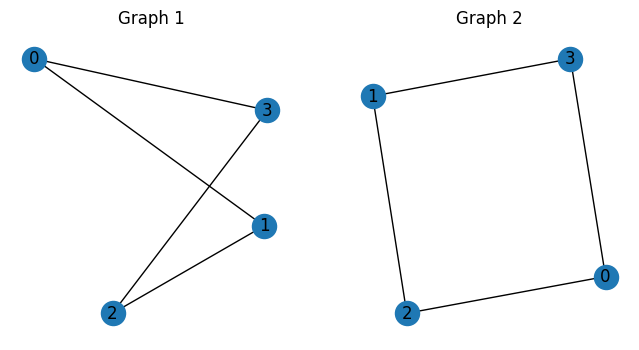
The input graphs are shown below.

# Create figure and subplots
fig, axs = plt.subplots(1, 2, figsize=(8, 4))

# Draw graphs
nx.draw(G1, ax=axs[0], with_labels=True)
axs[0].set_title("Graph 1")
nx.draw(G2, ax=axs[1], with_labels=True)
axs[1].set_title("Graph 2")

# Show the plot
plt.show()

Solve by JijZept's SA

We solve this problem using JijZept JijSASampler. We also use the parameter search function by setting search=True.

import jijzept as jz

# set sampler
sampler = jz.JijSASampler(config="../../../config.toml")
# solve problem
response = sampler.sample_model(problem, instance_data, multipliers={'const1-1': 0.3, 'const1-2': 0.3, 'const2': 0.3}, num_reads=100, search=True)

Check solution

In the end, we extract the lowest energy solution from the feasible solutions and check it.

# get sampleset
sampleset = response.get_sampleset()
# extract feasible samples
feasible_samples = sampleset.feasibles()
if len(feasible_samples) == 0:
    print("No feasible sample found ...")
else:
    # get feasible solution from samples
    feasible_solution = feasible_samples[0].var_values["x"].values
    # get vertex number and order
    vertices, orders = zip(*feasible_solution)
    print(f'vertex: {vertices}')
    print(f'orders: {orders}')

(0, 3) (2, 0) (3, 2) (1, 1)
vertex: (0, 2, 3, 1)
orders: (3, 0, 2, 1)

As we expected, JijZept successfully shows that it is isomorphic.